Cross-correlation#
Cross-correlation is a measure of similarity between two signals or datasets as a function of the time lag applied to one of them. It quantifies how much one signal or dataset matches a shifted version of another, indicating any time-dependent similarity.
Cross-correlation is critically important in various fields due to its ability to reveal time-dependent relationships and patterns that are not immediately obvious in raw data. As mentioned earlier, the Fourier Transform can be interpreted as a form of cross-correlation between the signal being analyzed and a set of sine and cosine waves.
The cross-correlation of the real discrete-time signals \( x[n] \) and \( y[n] \) is expressed as:
\[ R_{xy} [l] = \sum\limits_{n=-\infty}^{\infty} x[n] \, y[n - l] \]
Where \( l \) is a time lag between signals.
In order to calculate the cross-correlation, we shift one signal relative to the other by one sample at a time and calculate the measure of similarity for each lag. This measure of similarity at each lag is called the cross-correlation coefficient.
In practice, we deal with finite-length signals. For a finite signal of length \( N \):
- \( x[n] = 0 \) for \( n < 0 \)
- \( x[n] = 0 \) for \( n > N-1 \)
The cross-correlation equation then becomes:
Let's begin with two examples.
Auto-correlation example#
Consider the digital signal \( x[n] \):
\[ x[n] = [0,1,-1,3,-2,0] \]
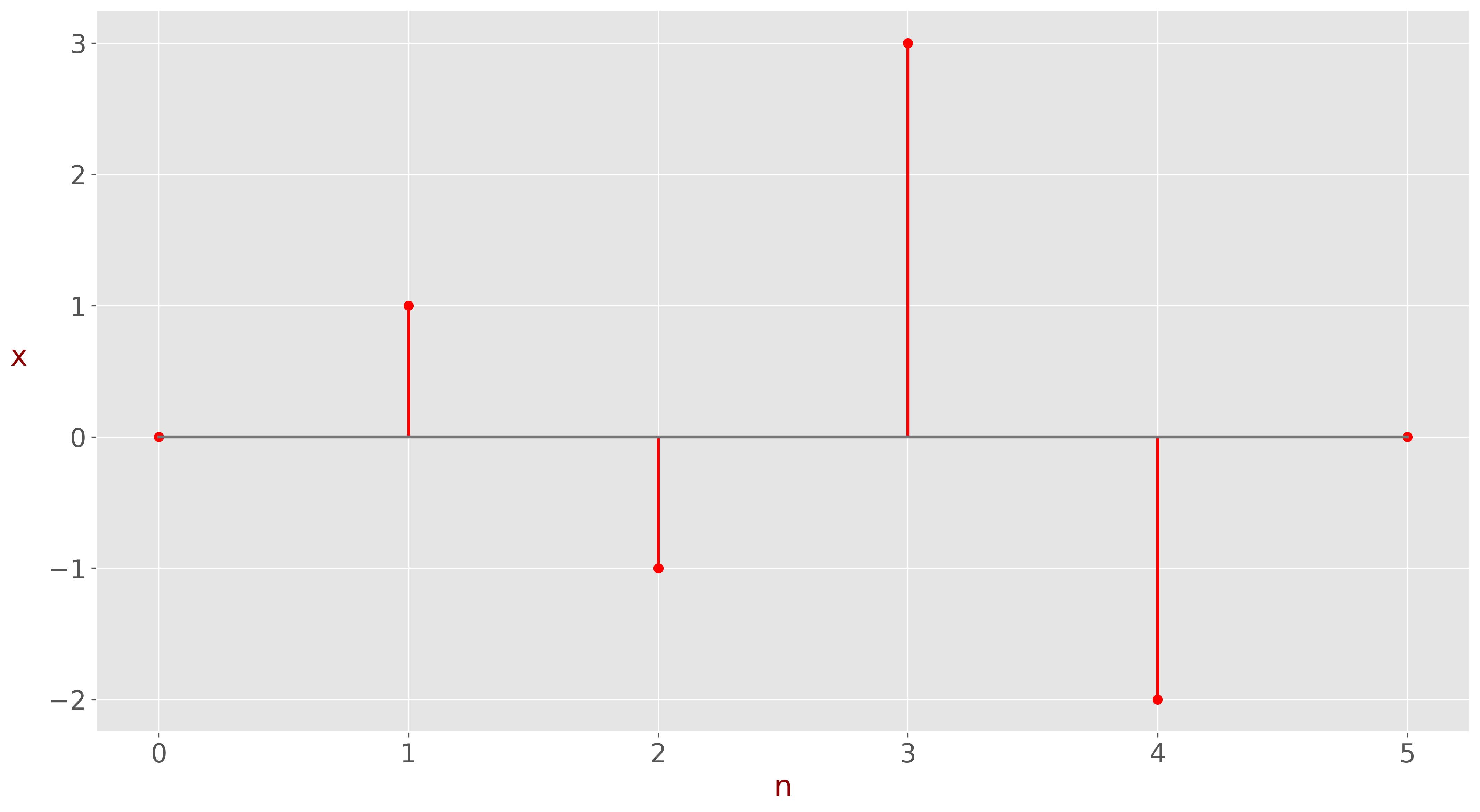
We will cross-correlate this signal with itself. The cross-correlation of a signal with itself is known as auto-correlation.
Auto-correlation is used to detect repeating patterns, periodic signals obscured by noise, and to understand the signal's temporal structure.
The cross-correlation equation becomes:
\[ R_{xx} [l] = \sum\limits_{n=l}^{N-1} x[n] x[n-l] \]
What should be the range of the time lag \( l \)?
For a finite signal of length \( N \), the summation is limited to the valid indices where both \( x[n] \) and \( x[n-l] \) are defined. The range of \( l \) (lags) depends on the length of the signal:
- Maximum Positive Lag: The maximum value of \( l \) is \( N-1 \).
- Maximum Negative Lag: The minimum value of \( l \) is \( -(N-1) \).
In our example, the signal has a length of \( N=6 \).
- \( l = -5 \)
The term \( x[n-l] \) corresponds to \( x[n+5] \)
\( x[n+5] \) is defined when \( 0 \leq n+5 \leq N-1 \), therefore \( -5 \leq n \leq 0 \)
\( x[n] \) is defined when \( 0 \leq n \leq N-1 \), therefore \( 0 \leq n \leq 5 \)
The only valid value for \( n \) is \( n = 0 \)
\[ R_{xx} [-5] = \sum\limits_{n=0}^{5} x[n] x[n+5] \]
\[ R_{xx} [-5] = \sum\limits_{n=0}^{0} x[n] x[n+5] \]
-
\( x[n] \) 0 1 -1 3 -2 0 \( x[n-l] \) 0 1 -1 3 -2 0 \( x[n] x[n-l] \) 0
\[ R_{xx} [-5] = x[0] \cdot x[5] = 0 \cdot 0 = 0 \]
- \( l = -4 \)
The term \( x[n-l] \) corresponds to \( x[n+4] \)
\( x[n+4] \) is defined when \( 0 \leq n+4 \leq N-1 \), therefore \( -4 \leq n \leq 1 \)
\( x[n] \) is defined when \( 0 \leq n \leq N-1 \), therefore \( 0 \leq n \leq 5 \)
The valid values for \( n \) are when \( 0 \leq n \leq 1 \)
\[ R_{xx} [-4] = \sum\limits_{n=0}^{5} x[n] x[n+4] \]
\[ R_{xx} [-4] = \sum\limits_{n=0}^{1} x[n] x[n+4] \]
-
\( x[n] \) 0 1 -1 3 -2 0 \( x[n-l] \) 0 1 -1 3 -2 0 \( x[n] x[n-l] \) 0 0
\[ R_{xx} [-4] = x[0] \cdot x[4] + x[1] \cdot x[5] = 0 \cdot (-2) + 1 \cdot 0 = 0 + 0 = 0 \]
- \( l = -3 \)
The term \( x[n-l] \) corresponds to \( x[n+3] \)
\( x[n+3] \) is defined when \( 0 \leq n+3 \leq N-1 \), therefore \( -3 \leq n \leq 2 \)
\( x[n] \) is defined when \( 0 \leq n \leq N-1 \), therefore \( 0 \leq n \leq 5 \)
The valid values for \( n \) are when \( 0 \leq n \leq 2 \)
\[ R_{xx} [-3] = \sum\limits_{n=0}^{2} x[n] x[n+3] \]
-
\( x[n] \) 0 1 -1 3 -2 0 \( x[n-l] \) 0 1 -1 3 -2 0 \( x[n] x[n-l] \) 0 -2 0
\[ R_{xx} [-3] = x[0] \cdot x[3] + x[1] \cdot x[4] + x[2] \cdot x[5] = 0 \cdot 3 + 1 \cdot (-2) + (-1) \cdot 0 = 0 - 2 + 0 = -2 \]
- \( l = -2 \)
The term \( x[n-l] \) corresponds to \( x[n+2] \)
\( x[n+2] \) is defined when \( 0 \leq n+2 \leq N-1 \), therefore \( -2 \leq n \leq 3 \)
\( x[n] \) is defined when \( 0 \leq n \leq N-1 \), therefore \( 0 \leq n \leq 5 \)
The valid values for \( n \) are when \( 0 \leq n \leq 3 \)
\[ R_{xx} [-2] = \sum\limits_{n=0}^{3} x[n] x[n+2] \]
-
\( x[n] \) 0 1 -1 3 -2 0 \( x[n-l] \) 0 1 -1 3 -2 0 \( x[n] x[n-l] \) 0 3 2 0
\[ \begin{aligned} R_{xx} [-2] &= x[0] \cdot x[2] + x[1] \cdot x[3] + x[2] \cdot x[4] + x[3] \cdot x[5] \\ &= 0 \cdot (-1) + 1 \cdot 3 + (-1) \cdot (-2) + 3 \cdot 0 \\ &= 0 + 3 + 2 + 0 = 5 \end{aligned} \]
- \( l = -1 \)
The term \( x[n-l] \) corresponds to \( x[n+1] \)
\( x[n+1] \) is defined when \( 0 \leq n+1 \leq N-1 \), therefore \( -1 \leq n \leq 4 \)
\( x[n] \) is defined when \( 0 \leq n \leq N-1 \), therefore \( 0 \leq n \leq 5 \)
The valid values for \( n \) are when \( 0 \leq n \leq 4 \)
\[ R_{xx} [-1] = \sum\limits_{n=0}^{4} x[n] x[n+1] \]
-
\( x[n] \) 0 1 -1 3 -2 0 \( x[n-l] \) 0 1 -1 3 -2 0 \( x[n] x[n-l] \) 0 -1 -3 -6 0
\[ \begin{aligned} R_{xx} [-1] &= x[0] \cdot x[1] + x[1] \cdot x[2] + x[2] \cdot x[3] + x[3] \cdot x[4] + x[4] \cdot x[5] \\ &= 0 \cdot 1 + 1 \cdot (-1) + (-1) \cdot 3 + 3 \cdot (-2) + (-2) \cdot 0 \\ &= 0 - 1 - 3 - 6 + 0 = -10 \end{aligned} \]
- \( l = 0 \)
The term \( x[n-l] \) corresponds to \( x[n] \)
\( x[n-0] \) is defined when \( 0 \leq n \leq N-1 \), therefore \( 0 \leq n \leq 5 \)
\( x[n] \) is defined when \( 0 \leq n \leq N-1 \), therefore \( 0 \leq n \leq 5 \)
The valid values for \( n \) are when \( 0 \leq n \leq 5 \)
\[ R_{xx} [0] = \sum\limits_{n=0}^{5} x[n] x[n] \]
-
\( x[n] \) 0 1 -1 3 -2 0 \( x[n-l] \) 0 1 -1 3 -2 0 \( x[n] x[n-l] \) 0 1 1 9 4 0
\[ \begin{aligned} R_{xx} [0] &= x[0] \cdot x[0] + x[1] \cdot x[1] + x[2] \cdot x[2] + x[3] \cdot x[3] + x[4] \cdot x[4] + x[5] \cdot x[5] \\ &= 0 \cdot 0 + 1 \cdot 1 + (-1) \cdot (-1) + 3 \cdot 3 + (-2) \cdot (-2) + 0 \cdot 0 \\ &= 0 + 1 + 1 + 9 + 4 + 0 = 15 \end{aligned} \]
- \( l = 1 \)
The term \( x[n-l] \) corresponds to \( x[n-1] \)
\( x[n-1] \) is defined when \( 0 \leq n-1 \leq N-1 \), therefore \( 1 \leq n \leq 6 \)
\( x[n] \) is defined when \( 0 \leq n \leq N-1 \), therefore \( 0 \leq n \leq 5 \)
The valid values for \( n \) are when \( 1 \leq n \leq 5 \)
\[ R_{xx} [1] = \sum\limits_{n=1}^{5} x[n] x[n-1] \]
-
\( x[n] \) 0 1 -1 3 -2 0 \( x[n-l] \) 0 1 -1 3 -2 0 \( x[n] x[n-l] \) 0 -1 -3 -6 0
\[ \begin{aligned} R_{xx} [1] &= x[1] \cdot x[0] + x[2] \cdot x[1] + x[3] \cdot x[2] + x[4] \cdot x[3] + x[5] \cdot x[4] \\ &= 1 \cdot 0 + (-1) \cdot 1 + 3 \cdot (-1) + (-2) \cdot 3 + 0 \cdot (-2) \\ &= 0 - 1 - 3 - 6 + 0 = -10 \end{aligned} \]
- \( l = 2 \)
The term \( x[n-l] \) corresponds to \( x[n-2] \)
\( x[n-2] \) is defined when \( 0 \leq n-2 \leq N-1 \), therefore \( 2 \leq n \leq 7 \)
\( x[n] \) is defined when \( 0 \leq n \leq N-1 \), therefore \( 0 \leq n \leq 5 \)
The valid values for \( n \) are when \( 2 \leq n \leq 5 \)
\[ R_{xx} [2] = \sum\limits_{n=2}^{5} x[n] x[n-2] \]
-
\( x[n] \) 0 1 -1 3 -2 0 \( x[n-l] \) 0 1 -1 3 -2 0 \( x[n] x[n-l] \) 0 3 2 0
\[ \begin{aligned} R_{xx} [2] &= x[2] \cdot x[0] + x[3] \cdot x[1] + x[4] \cdot x[2] + x[5] \cdot x[3] \\ &= (-1) \cdot 0 + 3 \cdot 1 + (-2) \cdot (-1) + 0 \cdot 3 \\ &= 0 + 3 + 2 + 0 = 5 \end{aligned} \]
- \( l = 3 \)
The term \( x[n-l] \) corresponds to \( x[n-3] \)
\( x[n-3] \) is defined when \( 0 \leq n-3 \leq N-1 \), therefore \( 3 \leq n \leq 8 \)
\( x[n] \) is defined when \( 0 \leq n \leq N-1 \), therefore \( 0 \leq n \leq 5 \)
The valid values for \( n \) are when \( 3 \leq n \leq 5 \)
\[ R_{xx} [3] = \sum\limits_{n=3}^{5} x[n] x[n-3] \]
-
\( x[n] \) 0 1 -1 3 -2 0 \( x[n-l] \) 0 1 -1 3 -2 0 \( x[n] x[n-l] \) 0 -2 0
\[ \begin{aligned} R_{xx} [3] &= x[3] \cdot x[0] + x[4] \cdot x[1] + x[5] \cdot x[2] \\ &= 3 \cdot 0 + (-2) \cdot 1 + 0 \cdot (-1) \\ &= 0 - 2 + 0 = -2 \end{aligned} \]
- \( l = 4 \)
The term \( x[n-l] \) corresponds to \( x[n-4] \)
\( x[n-4] \) is defined when \( 0 \leq n-4 \leq N-1 \), therefore \( 4 \leq n \leq 9 \)
\( x[n] \) is defined when \( 0 \leq n \leq N-1 \), therefore \( 0 \leq n \leq 5 \)
The valid values for \( n \) are when \( 4 \leq n \leq 5 \)
\[ R_{xx} [4] = \sum\limits_{n=4}^{5} x[n] x[n-4] \]
-
\( x[n] \) 0 1 -1 3 -2 0 \( x[n-l] \) 0 1 -1 3 -2 0 \( x[n] x[n-l] \) 0 0
\[ \begin{aligned} R_{xx} [4] &= x[4] \cdot x[0] + x[5] \cdot x[1] = (-2) \cdot 0 + 0 \cdot 1 = 0 + 0 = 0 \end{aligned} \]
- \( l = 5 \)
The term \( x[n-l] \) corresponds to \( x[n-5] \)
\( x[n-5] \) is defined when \( 0 \leq n-5 \leq N-1 \), therefore \( 5 \leq n \leq 10 \)
\( x[n] \) is defined when \( 0 \leq n \leq N-1 \), therefore \( 0 \leq n \leq 5 \)
The only valid value for \( n \) is \( n = 5 \)
\[ R_{xx} [5] = \sum\limits_{n=5}^{5} x[n] x[n-5] \]
-
\( x[n] \) 0 1 -1 3 -2 0 \( x[n-l] \) 0 1 -1 3 -2 0 \( x[n] x[n-l] \) 0
\[ \begin{aligned} R_{xx} [5] &= x[5] \cdot x[0] = 0 \cdot 0 = 0 \end{aligned} \]
The auto-correlation coefficients are:
| \( R_{xx}[-5] \) | \( R_{xx}[-4] \) | \( R_{xx}[-3] \) | \( R_{xx}[-2] \) | \( R_{xx}[-1] \) | \( R_{xx}[0] \) | \( R_{xx}[1] \) | \( R_{xx}[2] \) | \( R_{xx}[3] \) | \( R_{xx}[4] \) | \( R_{xx}[5] \) |
|---|---|---|---|---|---|---|---|---|---|---|
| 0 | 0 | -2 | 5 | -10 | 15 | -10 | 5 | -2 | 0 | 0 |
Normalization
Let us normalize the result. The cross-correlation normalization factor is given by:
\[ \frac{1}{\sqrt{\sum\limits_{k=-\infty}^{\infty} x_n^2} \sqrt{\sum\limits_{k=-\infty}^{\infty} y_n^2}} \]
For auto-correlation, the normalization factor becomes:
\[ \frac{1}{\sqrt{\sum\limits_{k=-\infty}^{\infty} x_n^2} \sqrt{\sum\limits_{k=-\infty}^{\infty} x_n^2}} = \frac{1}{\sum\limits_{k=-\infty}^{\infty} x_n^2} = \frac{1}{15} \]
The normalized auto-correlation coefficients are:
| \( R_{xx}[-5] \) | \( R_{xx}[-4] \) | \( R_{xx}[-3] \) | \( R_{xx}[-2] \) | \( R_{xx}[-1] \) | \( R_{xx}[0] \) | \( R_{xx}[1] \) | \( R_{xx}[2] \) | \( R_{xx}[3] \) | \( R_{xx}[4] \) | \( R_{xx}[5] \) |
|---|---|---|---|---|---|---|---|---|---|---|
| 0 | 0 | \(\displaystyle -\frac{2}{15} \) | \(\displaystyle \frac{1}{3} \) | \(\displaystyle -\frac{2}{3} \) | 1 | \(\displaystyle -\frac{2}{3} \) | \(\displaystyle \frac{1}{3} \) | \(\displaystyle -\frac{2}{15} \) | 0 | 0 |
As expected, the auto-correlation peak occurs at zero-time lag. The signals are identical at this point, since \( R_{xx}[0] = 1 \).
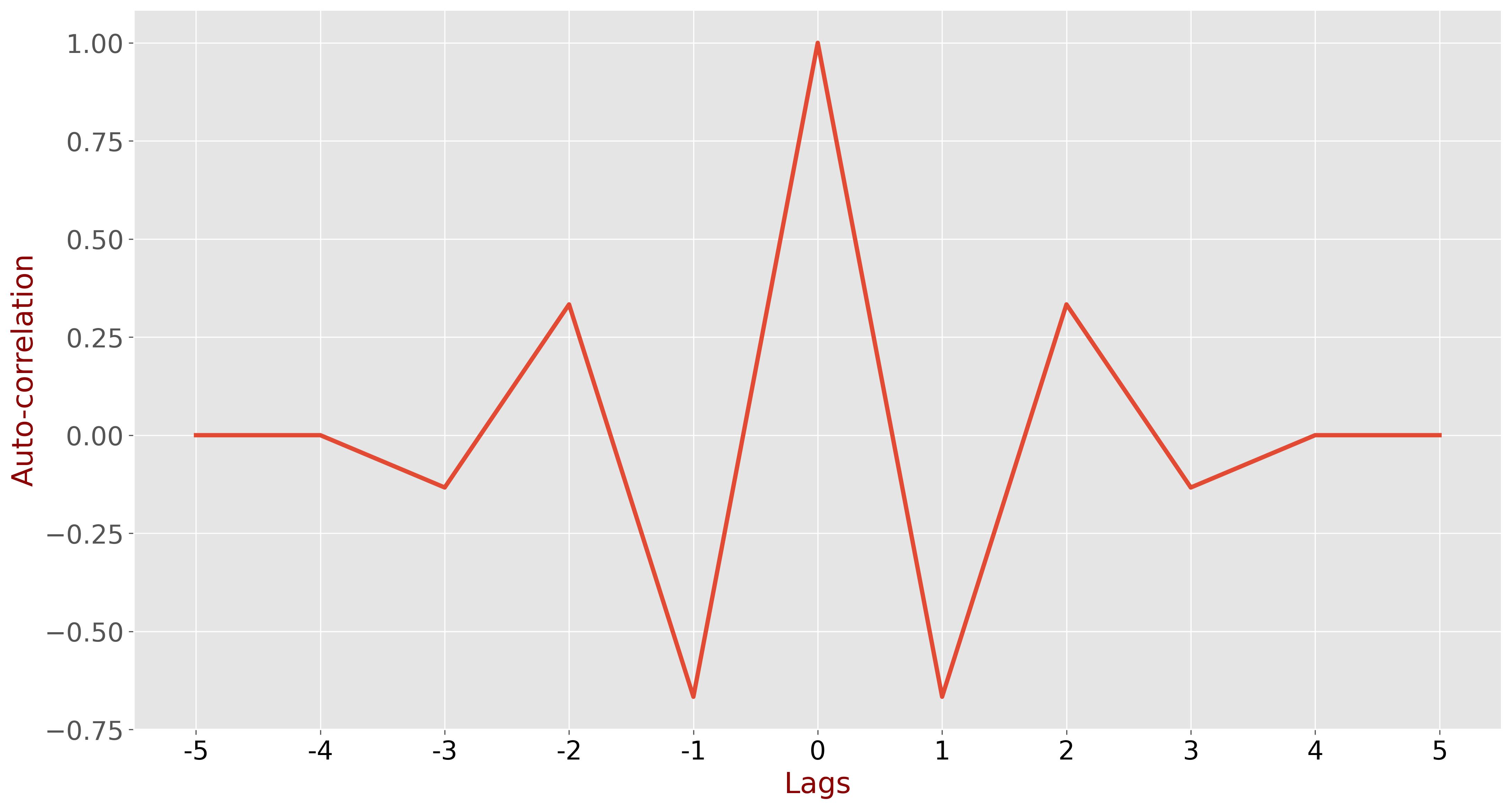
As you can see, the auto-correlation function is even – the right part is similar to the left part. Therefore, we can save on computation by calculating only \( N \) indices of the auto-correlation instead of \( 2N-1 \).
Cross-correlation example#
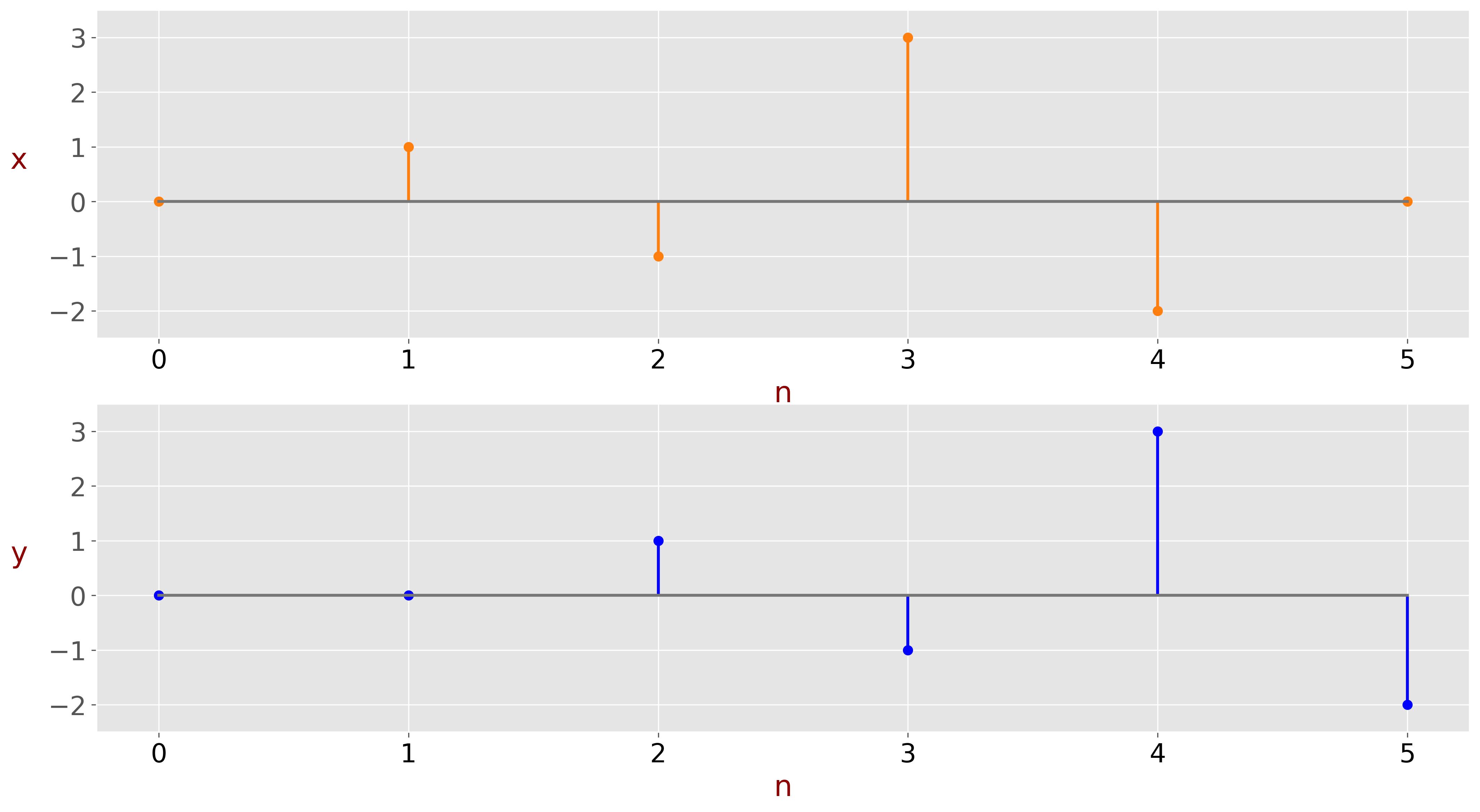
Let us cross-correlate the digital signal \( x[n] \) with its lagged copy:
\[ x[n] = [0,1,-1,3,-2,0] \] \[ y[n] = [0,0,1,-1,3,-2] \]
In our example, the signal has a length of \( N = 6 \).
Cross-correlation calculations
-
\( l = -5 \)
\[ R_{xy} [-5] = \sum\limits_{n=0}^{0} x[n] y[n+5] \]
-
\( x[n] \) 0 1 -1 3 -2 0 \( y[n-l] \) 0 0 1 -1 3 -2 \( x[n] x[n-l] \) 0
\[ \begin{aligned} R_{xy} [-5] &= x[0] \cdot y[5] = 0 \cdot (-2) = 0 \end{aligned} \]
-
\( l = -4 \)
\[ R_{xy} [-4] = \sum\limits_{n=0}^{1} x[n] y[n+4] \]
-
\( x[n] \) 0 1 -1 3 -2 0 \( y[n-l] \) 0 0 1 -1 3 -2 \( x[n] y[n-l] \) 0 -2
\[ \begin{aligned} R_{xy} [-4] &= x[0] \cdot y[4] + x[1] \cdot y[5] = 0 \cdot 3 + 1 \cdot (-2) = -2 \end{aligned} \]
-
\( l = -3 \)
\[ R_{xy} [-3] = \sum\limits_{n=0}^{2} x[n] y[n+3] \]
-
\( x[n] \) 0 1 -1 3 -2 0 \( y[n-l] \) 0 0 1 -1 3 -2 \( x[n] y[n-l] \) 0 3 2
\[ \begin{aligned} R_{xy} [-3] &= x[0] \cdot y[3] + x[1] \cdot y[4] + x[2] \cdot y[5] \\ &= 0 \cdot (-1) + 1 \cdot 3 + (-1) \cdot (-2) = 5 \end{aligned} \]
-
\( l = -2 \)
\[ R_{xy} [-2] = \sum\limits_{n=0}^{3} x[n] y[n+2] \]
-
\( x[n] \) 0 1 -1 3 -2 0 \( y[n-l] \) 0 0 1 -1 3 -2 \( x[n] y[n-l] \) 0 -1 -3 -6
\[ \begin{aligned} R_{xy} [-2] &= x[0] \cdot y[2] + x[1] \cdot y[3] + x[2] \cdot y[4] + x[3] \cdot y[5] \\ &= 0 \cdot 1 + 1 \cdot (-1) + (-1) \cdot 3 + 3 \cdot (-2) = -10 \end{aligned} \]
-
\( l = -1 \)
\[ R_{xy} [-1] = \sum\limits_{n=0}^{4} x[n] y[n+1] \]
-
\( x[n] \) 0 1 -1 3 -2 0 \( y[n-l] \) 0 0 1 -1 3 -2 \( x[n] y[n-l] \) 0 1 1 9 4
\[ \begin{aligned} R_{xy} [-1] &= x[0] \cdot y[1] + x[1] \cdot y[2] + x[2] \cdot y[3] + x[3] \cdot y[4] + x[4] \cdot y[5] \\ &= 0 \cdot 0 + 1 \cdot 1 + (-1) \cdot (-1) + 3 \cdot 3 + (-2) \cdot (-2) = 15 \end{aligned} \]
-
\( l = 0 \)
\[ R_{xy} [0] = \sum\limits_{n=0}^{5} x[n] y[n] \]
-
\( x[n] \) 0 1 -1 3 -2 0 \( y[n-l] \) 0 0 1 -1 3 -2 \( x[n] y[n-l] \) 0 0 -1 -3 -6 0
\[ \begin{aligned} R_{xy} [0] &= x[0] \cdot y[0] + x[1] \cdot y[1] + x[2] \cdot y[2] + x[3] \cdot y[3] + x[4] \cdot y[4] + x[5] \cdot y[5] \\ &= 0 \cdot 0 + 1 \cdot 0 + (-1) \cdot 1 + 3 \cdot (-1) + (-2) \cdot 3 + 0 \cdot (-2) = -10 \end{aligned} \]
-
\( l = 1 \)
\[ R_{xy} [1] = \sum\limits_{n=1}^{5} x[n] y[n-1] \]
-
\( x[n] \) 0 1 -1 3 -2 0 \( y[n-l] \) 0 0 1 -1 3 -2 \( x[n] y[n-l] \) 0 0 3 2 0
\[ \begin{aligned} R_{xy} [1] &= x[1] \cdot y[0] + x[2] \cdot y[1] + x[3] \cdot y[2] + x[4] \cdot y[3] + x[5] \cdot y[4] \\ &= 1 \cdot 0 + (-1) \cdot 0 + 3 \cdot 1 + (-2) \cdot (-1) + 0 \cdot 3 = 5 \end{aligned} \]
-
\( l = 2 \)
\[ R_{xy} [2] = \sum\limits_{n=2}^{5} x[n] y[n-2] \]
-
\( x[n] \) 0 1 -1 3 -2 0 \( y[n-l] \) 0 0 1 -1 3 -2 \( x[n] y[n-l] \) 0 0 -2 0
\[ \begin{aligned} R_{xy} [2] &= x[2] \cdot y[0] + x[3] \cdot y[1] + x[4] \cdot y[2] + x[5] \cdot y[3] \\ &= (-1) \cdot 0 + 3 \cdot 0 + (-2) \cdot 1 + 0 \cdot (-1) = -2 \end{aligned} \]
-
\( l = 3 \)
\[ R_{xy} [3] = \sum\limits_{n=3}^{5} x[n] y[n-3] \]
-
\( x[n] \) 0 1 -1 3 -2 0 \( y[n-l] \) 0 0 1 -1 3 -2 \( x[n] y[n-l] \) 0 0 0
\[ \begin{aligned} R_{xy} [3] &= x[3] \cdot y[0] + x[4] \cdot y[1] + x[5] \cdot y[2] \\ &= 3 \cdot 0 + (-2) \cdot 0 + 0 \cdot 1 = 0 \end{aligned} \]
-
\( l = 4 \)
\[ R_{xy} [4] = \sum\limits_{n=4}^{5} x[n] y[n-4] \]
-
\( x[n] \) 0 1 -1 3 -2 0 \( y[n-l] \) 0 0 1 -1 3 -2 \( x[n] y[n-l] \) 0 0
\[ \begin{aligned} R_{xy} [4] &= x[4] \cdot y[0] + x[5] \cdot y[1] = (-2) \cdot 0 + 0 \cdot 0 = 0 \end{aligned} \]
-
\( l = 5 \)
\[ R_{xy} [5] = \sum\limits_{n=5}^{5} x[n] y[n-5] \]
-
\( x[n] \) 0 1 -1 3 -2 0 \( y[n-l] \) 0 0 1 -1 3 -2 \( x[n] y[n-l] \) 0
\[ \begin{aligned} R_{xy} [5] &= x[5] \cdot y[0] = 0 \cdot 0 = 0 \end{aligned} \]
The auto-correlation coefficients are:
| \( R_{xx}[-5] \) | \( R_{xx}[-4] \) | \( R_{xx}[-3] \) | \( R_{xx}[-2] \) | \( R_{xx}[-1] \) | \( R_{xx}[0] \) | \( R_{xx}[1] \) | \( R_{xx}[2] \) | \( R_{xx}[3] \) | \( R_{xx}[4] \) | \( R_{xx}[5] \) |
|---|---|---|---|---|---|---|---|---|---|---|
| 0 | -2 | 5 | -10 | 15 | -10 | 5 | -2 | 0 | 0 | 0 |
Normalization
Let us normalize the result. The cross-correlation normalization factor is given by:
\[ \frac{1}{\sqrt{\sum\limits_{k=-\infty}^{\infty} x_n^2} \sqrt{\sum\limits_{k=-\infty}^{\infty} y_n^2}} = \frac{1}{15} \]
The normalized auto-correlation coefficients are:
| \( R_{xx}[-5] \) | \( R_{xx}[-4] \) | \( R_{xx}[-3] \) | \( R_{xx}[-2] \) | \( R_{xx}[-1] \) | \( R_{xx}[0] \) | \( R_{xx}[1] \) | \( R_{xx}[2] \) | \( R_{xx}[3] \) | \( R_{xx}[4] \) | \( R_{xx}[5] \) |
|---|---|---|---|---|---|---|---|---|---|---|
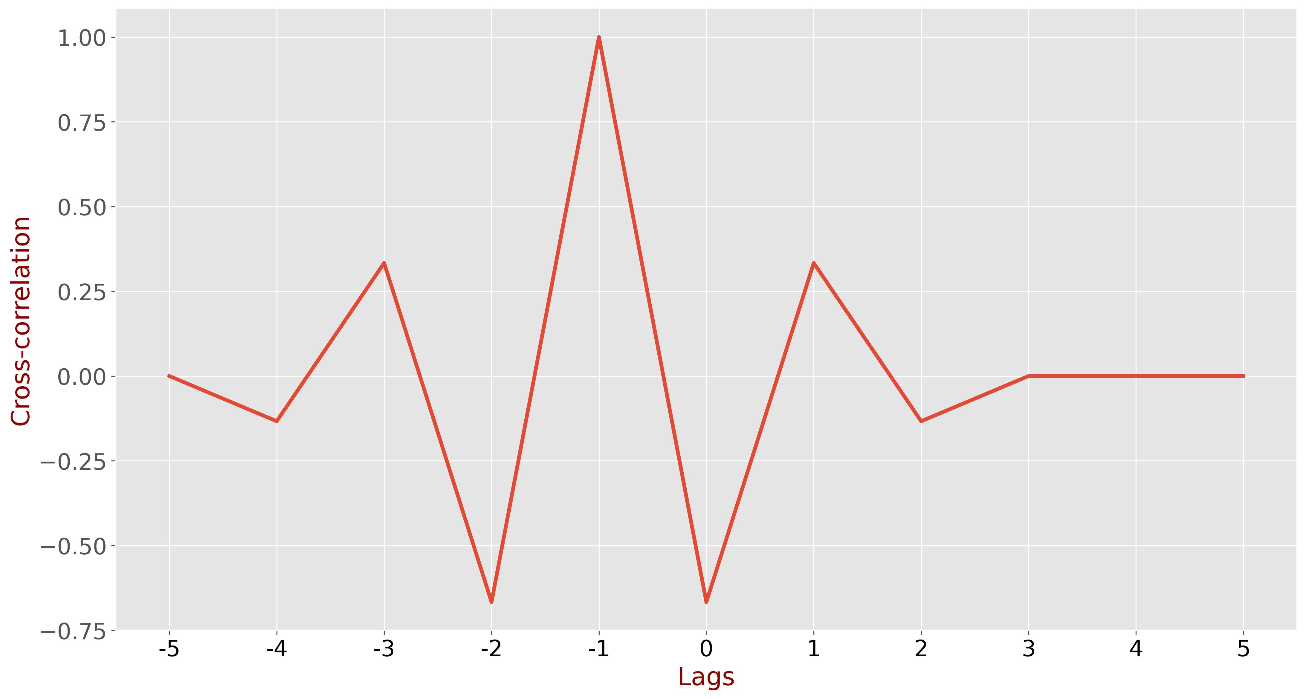
| 0 | \(\displaystyle -\frac{2}{15} \) | \(\displaystyle \frac{1}{3} \) | \(\displaystyle -\frac{2}{3} \) | 1 | \(\displaystyle -\frac{2}{3} \) | \(\displaystyle \frac{1}{3} \) | \(\displaystyle -\frac{2}{15} \) | 0 | 0 | 0 |
As expected, the cross-correlation peak occurs at a one-tap lag. At this point, the signals are identical since \( y[n] \) is a one-tap lagged copy of \( x[n] \).
Fast Computation Method#
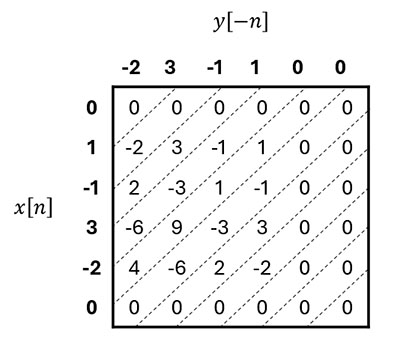
To compute cross-correlation efficiently, you can create a matrix where each cell contains the product of \( x[n] \) and \( y[-n] \), where \( y[-n] \) is the time-reversed version of \( y[n] \). The cross-correlation coefficients can then be obtained by summing the elements along the diagonals of this matrix.
| \( R_{xx}[-5] \) | \( R_{xx}[-4] \) | \( R_{xx}[-3] \) | \( R_{xx}[-2] \) | \( R_{xx}[-1] \) | \( R_{xx}[0] \) | \( R_{xx}[1] \) | \( R_{xx}[2] \) | \( R_{xx}[3] \) | \( R_{xx}[4] \) | \( R_{xx}[5] \) |
|---|---|---|---|---|---|---|---|---|---|---|
| 0 | -2 | 5 | -10 | 15 | -10 | 5 | -2 | 0 | 0 | 0 |
Cross-correlation of continuous signals#
While the cross-correlation of discrete-time signals can be implemented in software or digital hardware, the cross-correlation of continuous-time signals remains theoretical and is primarily used for mathematical derivations. In the continuous-time domain, the summation transforms into an integral, and the cross-correlation of a real periodic signal over period \( T \) is represented as follows:
Where:
- \( \tau \) is a time delay between functions
- \( \frac{1}{T} \) is a normalization factor over period \( T \)
Let us cross-correlate a sine function \( A \sin(\omega t) \) with its leading copy \( A \sin(\omega t + \phi) \), where:
- \( A \) is an amplitude
- \( \omega \) is an angular frequency
- \( \phi \) is a phase shift
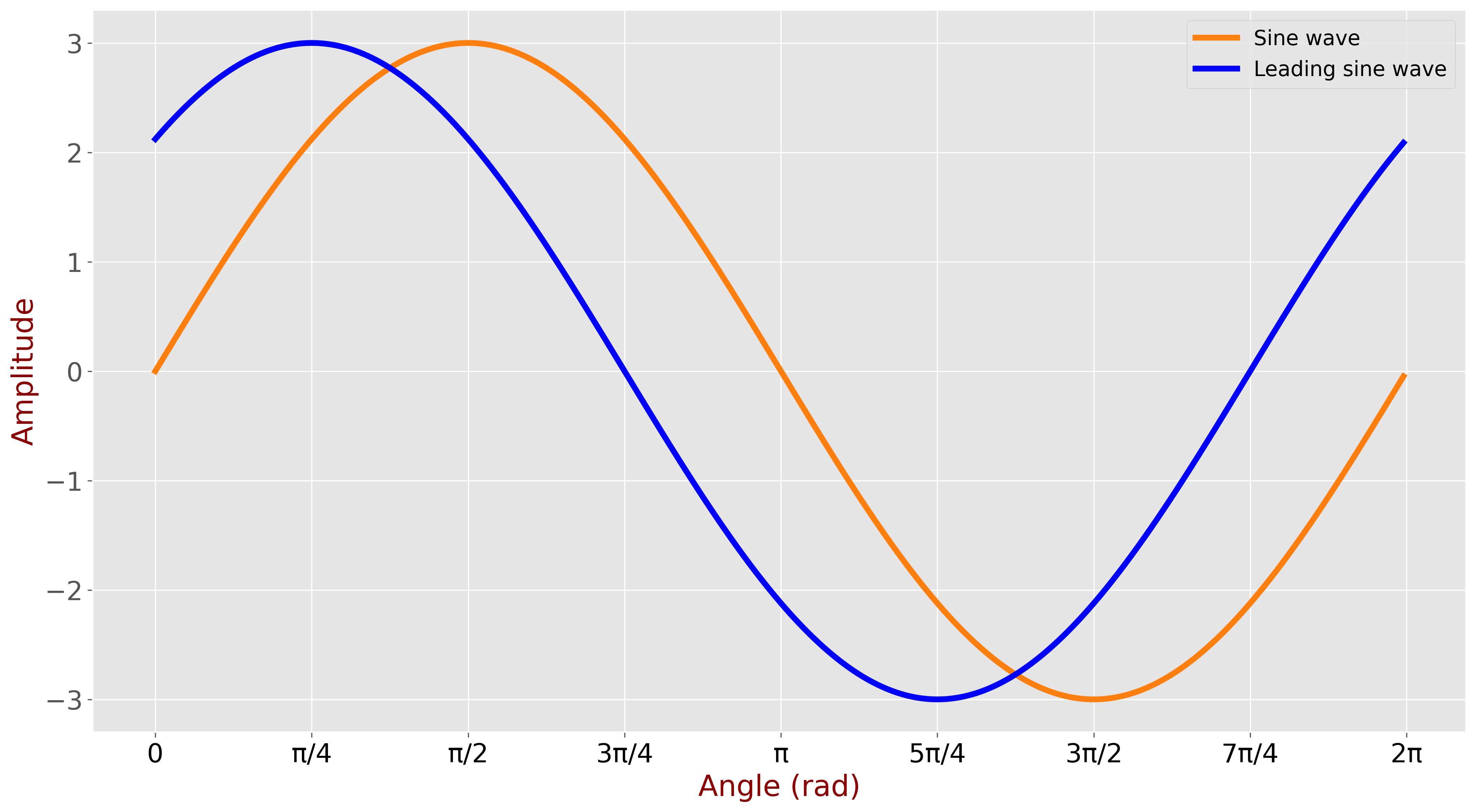
The cross-correlation coefficients can be found by solving:
\[ R_{xy} (\tau) = \frac{1}{T} \int\limits_{-T/2}^{T/2} A \sin(\omega t) A \sin(\omega (t-\tau) + \phi) \, dt \]Solving the integral yields:
See Appendix A for the integral solution.
This result shows that the cross-correlation between \( \sin(\omega t) \) and its leading copy \( \sin(\omega t + \phi) \) is a scaled cosine function of the phase shift and the delay \( \tau \).
Let us analyze the result. The cross-correlation function \( R_{xy} (\tau) \) reaches the maximum when \( \cos(\omega \tau - \phi) = 1 \), therefore:
\[ \max\limits_{\tau} R_{xy} (\tau), \quad \text{when } \omega \tau = \phi \]When the original sine function \( A \sin(\omega t) \) is shifted by \( \phi \), it becomes similar to its leading copy \( A \sin(\omega t + \phi) \).
Remember that the angular frequency \( \omega \) [rad/s] multiplied by time-lag \( \tau \) [s] yields the angle (phase) shift.
The term \( \dfrac{A^2}{2} \) represents the average power of a sinusoidal signal (see Appendix D for details). The value of the cross-correlation function of a sinusoidal signal at its maximum represents the signal's average power, and this is an important conclusion that we will use later.
The following figure exemplifies the cross-correlation of a sine wave with amplitude \( A=3 \) with its leading copy, where phase difference equals \( \dfrac{\pi}{4} \) (45 degrees).
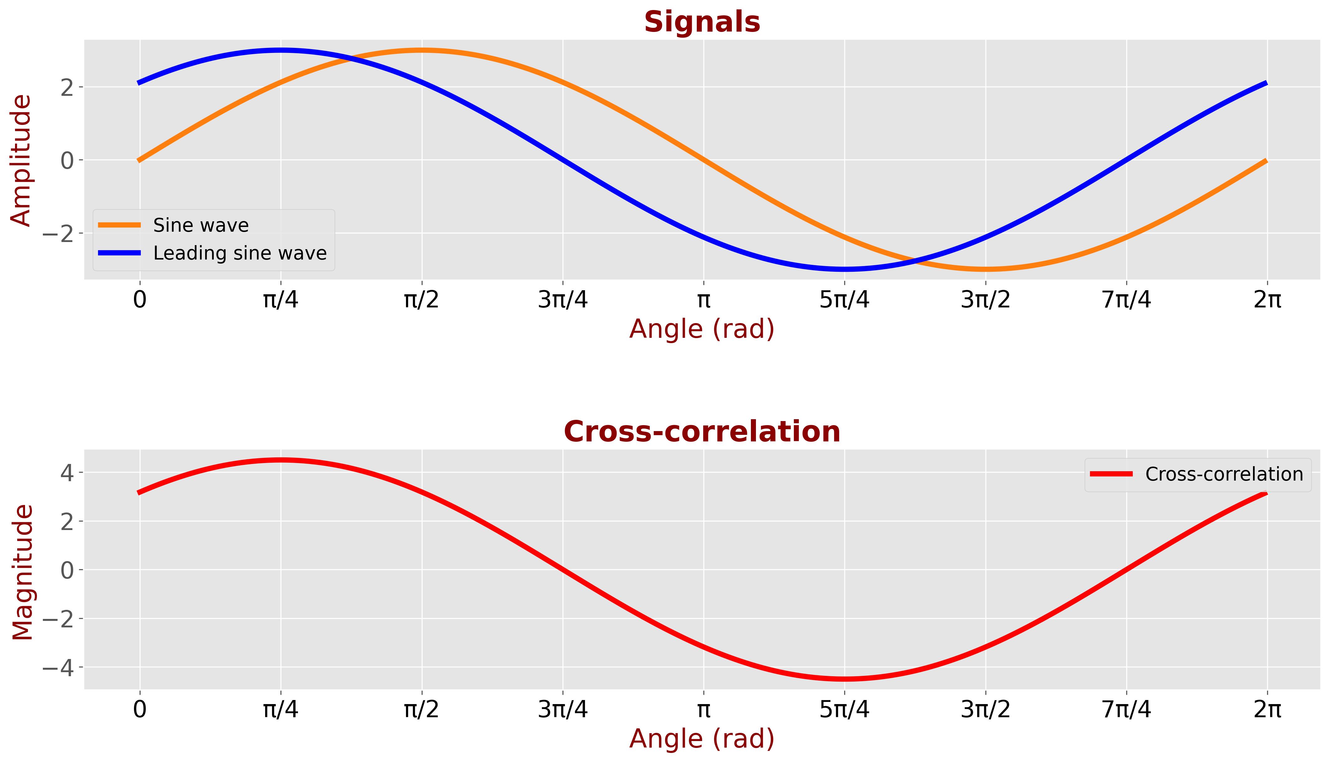
We can see that the cross-correlation peaks at an angle \( \dfrac{\pi}{4} \), while the peak magnitude equals \( \dfrac{A^2}{2} = 4.5 \).