DFT Example Software Implementation
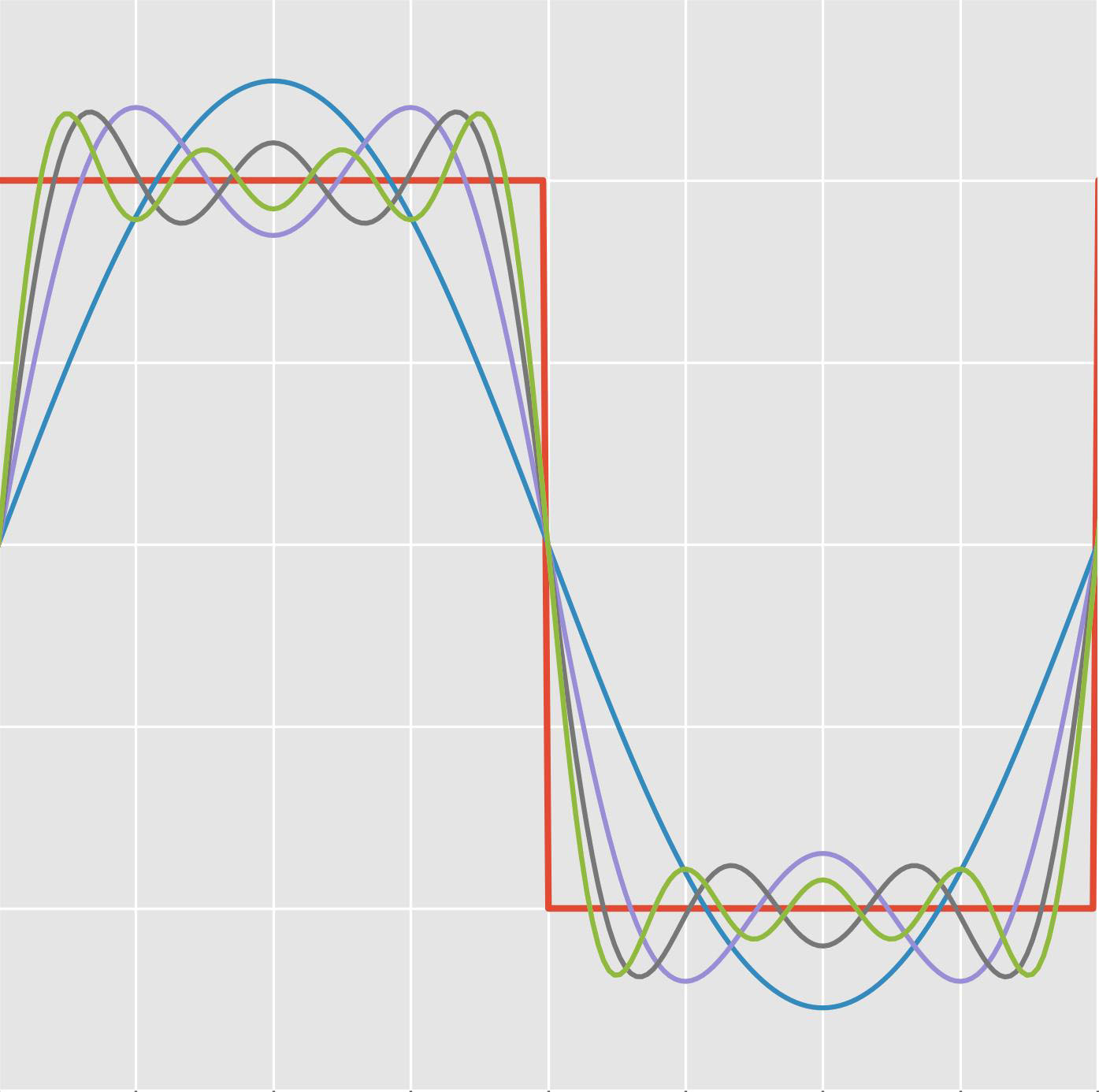
This section demonstrates the implementation of a previously solved example in MATLAB, Python, and C. It reconstructs the input signal - comprising a DC component and two sinusoidal components, computes its Discrete Fourier Transform, analyzes the resulting frequency components (amplitudes and phases), and visualizes the results.
MATLAB#
%% Create Input Signal
% Define input components: DC and two sinusoidal signals
A = [-1 3 2]; % Amplitudes (V)
f = [0 1 3]; % Frequencies (Hz)
phi = [pi/2 pi/4 0]; % Phases (rad)
T = 1; % Signal duration (s)
fs = 8; % Sampling frequency (Hz)
% Create sampled signal
N = T * fs; % Number of samples
n = (0 : N-1)'; % Sample indices
% Initialize signal array
x = zeros(N, 1);
% Construct the signal as a sum of sinusoids
for i = 1 : length(A)
x = x + A(i) * sin(2 * pi * f(i) * n / fs + phi(i));
end
%% Compute DFT
[a, b] = dft(x); % Compute DFT
% Set very small values to 0 to mitigate numerical errors
threshold = 1e-10;
a(abs(a) < threshold) = 0;
b(abs(b) < threshold) = 0;
%% Analyze Frequency Components
Amp = sqrt(a.^2 + b.^2); % Compute amplitude of signal components
Amp(1) = a(1) / 2; % DC component amplitude correction
phase = atan(a./b); % Compute phase (corrected formula)
phase(1) = NaN; % Set DC component phase to NaN
% Frequency axis adjustment for visualization
frq = (-N/2 : N/2-1) / N * fs;
Amp = fftshift(Amp); % Rearrange amplitudes for proper frequency order
phase = fftshift(phase); % Rearrange phases for proper frequency order
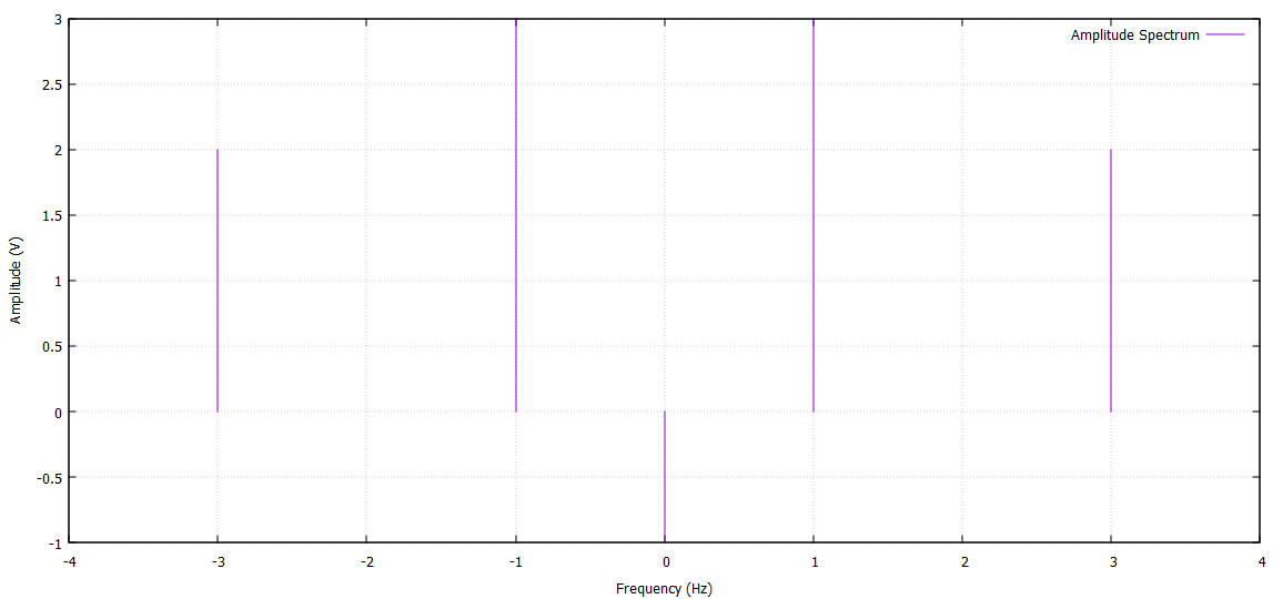
%% Plot Amplitude and Phase Spectra
figure;
subplot(2,1,1);
stem(frq, Amp, 'filled');
xlabel('Frequency (Hz)'); ylabel('Amplitude (V)');
title('Amplitude Spectrum'); grid on;
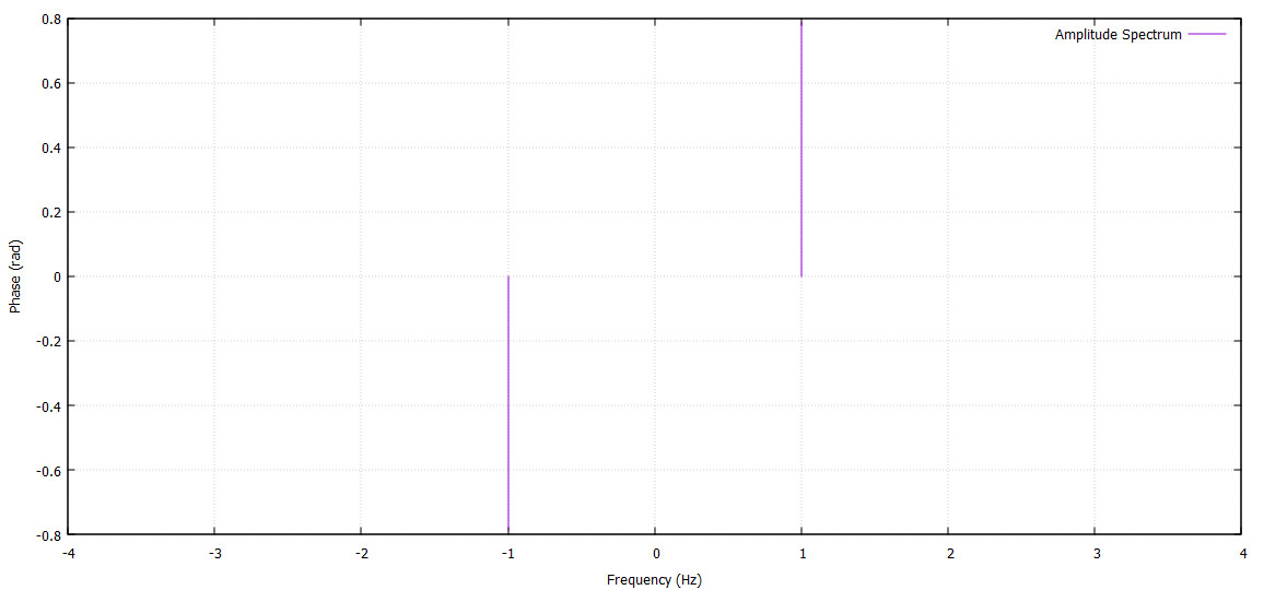
subplot(2,1,2);
stem(frq, phase, 'filled');
xlabel('Frequency (Hz)'); ylabel('Phase (rad)');
title('Phase Spectrum'); grid on;
%% DFT Function Implementation
function [a, b] = dft(x)
% Compute the Discrete Fourier Transform (DFT) of a real input signal
N = length(x); % Number of samples
n = 0 : N-1; % Sample indices
phi = 2 * pi * (n' * n) / N; % Compute angles for DFT matrix
% Compute cosine and sine frequency components
a = (2 / N) * cos(phi) * x;
b = (2 / N) * sin(phi) * x;
end
Python#
import numpy as np
import matplotlib.pyplot as plt

# Create Input Signal

# Define input components: DC and two sinusoidal signals
A = np.array([-1, 3, 2])     # Amplitudes (V)
f = np.array([0, 1, 3])      # Frequencies (Hz)
phi = np.array([np.pi/2, np.pi/4, 0])  # Phases (rad)

T = 1    # Signal duration (s)
fs = 8   # Sampling frequency (Hz)

# Create sampled signal
N = int(T * fs)    # Number of samples
n = np.arange(N)   # Sample indices

# Initialize signal array
x = np.zeros(N)

# Construct the signal as a sum of sinusoids
for i in range(len(A)):
    x += A[i] * np.sin(2 * np.pi * f[i] * n / fs + phi[i])

# Compute DFT
def dft(x):
    """ Compute the Discrete Fourier Transform (DFT) of a real input signal. """
    N = len(x)
    n = np.arange(N).reshape(1, N) # Create row vector
    phi = 2 * np.pi * n.T * n / N  # Compute angles for DFT matrix

    # Compute cosine and sine frequency components
    a = (2 / N) * np.dot(np.cos(phi), x)
    b = (2 / N) * np.dot(np.sin(phi), x)
    return a, b

a, b = dft(x)  # Compute DFT

# Set very small values to 0 to mitigate numerical errors
threshold = 1e-10
a[np.abs(a) < threshold] = 0
b[np.abs(b) < threshold] = 0

# Analyze Frequency Components
Amp = np.sqrt(a**2 + b**2)   # Compute amplitude of signal components
Amp[0] = a[0] / 2            # DC component amplitude correction

phase = np.arctan(a/b)       # Compute phase (corrected formula)
phase[0] = np.nan            # Set DC component phase to NaN

# Frequency axis adjustment for visualization
frq = np.fft.fftfreq(N, d=1/fs)  # Compute frequency axis
frq = np.fft.fftshift(frq)       # Rearrange for plotting
Amp = np.fft.fftshift(Amp)       # Rearrange amplitudes
phase = np.fft.fftshift(phase)   # Rearrange phases

# Plot Amplitude and Phase Spectra
plt.figure(figsize=(10, 6))

plt.subplot(2, 1, 1)
markerline, stemline, baseline = plt.stem(frq, Amp, linefmt='b', markerfmt='bo', basefmt="k-")
plt.xlabel('Frequency (Hz)')
plt.ylabel('Amplitude (V)')
plt.title('Amplitude Spectrum')
plt.grid()

plt.subplot(2, 1, 2)
markerline, stemline, baseline = plt.stem(frq, phase, linefmt='r', markerfmt='ro', basefmt="k-")
plt.xlabel('Frequency (Hz)')
plt.ylabel('Phase (rad)')
plt.title('Phase Spectrum')
plt.grid()

plt.tight_layout()
plt.show()
C#
The C code was developed using the Code::Blocks IDE as a Console Application. The results are stored in .dat files, which can be visualized using GNUplot for analysis and comparison.
#include <stdio.h>
#include <stdlib.h.h>
#include <math.h>

#define PI 3.14159265358979323846
#define FS 8        // Sampling frequency (Hz)
#define T 1         // Signal duration (s)
//#define N (FS * T)  // Number of samples


// DFT Function
void dft(double x[], double a[], double b[], int N) {
    // Compute DFT of a real input signal
    for (int k = 0; k < N; k++) {
        a[k] = 0.0;
        b[k] = 0.0;
        for (int n = 0; n < N; n++) {
            double phi = 2 * PI * k * n / N;
            a[k] += (2.0 / N) * x[n] * cos(phi);
            b[k] += (2.0 / N) * x[n] * sin(phi);
        }
    }
}

// FFT Shift (Rearrange Frequency Components)
void fftshift(double arr[], int N) {
    int half = N / 2;
    double temp;

    for (int i = 0; i < half; i++) {
        temp = arr[i];
        arr[i] = arr[i + half];
        arr[i + half] = temp;
    }
}

int main() {
    int N = FS * T; // Number of samples
    int L;          // Number of input signals

    // Define input components: DC and two sinusoidal signals
    double A[] = {-1, 3, 2};          // Amplitudes (V)
    double f[] = {0, 1, 3};           // Frequencies (Hz)
    double phi[] = {PI/2, PI/4, 0};   // Phases (rad)

    double x[N];                      // Sampled signal array
    double a[N], b[N];                // DFT cosine and sine coefficients
    double Amp[N], phase[N], frq[N];  // Amplitude and phase spectra

    // Generate sampled signal
    L = sizeof(A) / sizeof(A[0]);
    for (int n = 0; n < N; n++) {
        x[n] = 0;
        for (int i = 0; i < L; i++) {
            x[n] += A[i] * sin(2 * PI * f[i] * n / FS + phi[i]);
        }
    }

    // Compute DFT
    dft(x, a, b, N);

    // Eliminate very small numerical errors
    for (int k = 0; k < N; k++) {
        if (fabs(a[k]) < 1e-10) a[k] = 0;
        if (fabs(b[k]) < 1e-10) b[k] = 0;
    }

    // Compute amplitude and phase spectra
    for (int k = 0; k < N; k++) {
        Amp[k] = sqrt(a[k] * a[k] + b[k] * b[k]);  // Magnitude
        if (k == 0) {
            Amp[k] = a[k] / 2;  // DC component correction
            phase[k] = 0;       // DC phase is undefined
        } else {
            if (b[k] == 0) {
                phase[k] = 0;   // Division by 0
            } else {
                phase[k] = atan(a[k]/b[k]);  // Compute phase
            }
        }
    }

    // Frequency axis
    for (int k = 0; k < N; k++) {
        frq[k] = ((k - N / 2) * FS) / (double)N;
    }

    // Apply FFT Shift to rearrange amplitude and phase spectra
    fftshift(Amp, N);
    fftshift(phase, N);


    // Print results
    printf("Amplitude values:\n");
    for (int i = 0; i < N; i++) {
        printf("Amplitude[%d] = %f\n", i, Amp[i]);
    }

    printf("\nPhase values:\n");
    for (int i = 0; i < N; i++) {
        printf("Phase[%d] = %f\n", i, phase[i]);
    }

    printf("\nFrequencies:\n");
    for (int i = 0; i < N; i++) {
        printf("Frequency[%d] = %f\n", i, frq[i]);
    }

    // Save data to files for later visualization
    FILE *amp_file = fopen("amplitude_spectrum.dat", "w");
    FILE *phase_file = fopen("phase_spectrum.dat", "w");

    for (int k = 0; k < N; k++) {
        fprintf(amp_file, "%lf %lf\n", frq[k], Amp[k]);
        fprintf(phase_file, "%lf %lf\n", frq[k], phase[k]);
    }

    fclose(amp_file);
    fclose(phase_file);

    // visualize
    printf("\nUse GNUplot to visualize:\n");
    printf("gnuplot -e \"plot 'amplitude_spectrum.dat' with linespoints title 'Amplitude Spectrum'\"\n");
    printf("gnuplot -e \"plot 'phase_spectrum.dat' with linespoints title 'Phase Spectrum'\"\n");

    return 0;
}
Visualization
- Open command prompt (Windows)
- Check if GNUplot is installed using:
- Navigate to the folder with '.dat' files using 'cd' command:
- If the folder is on a different drive (e.g., D:), first switch to that drive:
- Verify the files exist by listing them:
- Open GNUplot by running:
- To plot the Amplitude Spectrum, type inside the GNUplot interface:
- To plot the Phase Spectrum, type inside the GNUplot interface:
- To plot both graphs in one window:
- To save the Amplitude Spectrum in the current directory, type inside the GNUplot interface:
- To exit GNUplot, type:
where gnuplot
or
gnuplot --version
If GNUplot is not installed, download and install it, ensuring the "Add to system PATH" option is selected during installation.
cd C:\path\to\your\folder
Replace 'C:\path\to\your\folder' with the actual folder path.
D:

cd path\to\your\folder
dir
gnuplot
This should open the GNUplot command-line interface.
set xlabel 'Frequency (Hz)'
set ylabel 'Amplitude (V)'
set grid
plot 'amplitude_spectrum.dat' with impulses title 'Amplitude Spectrum'
set xlabel 'Frequency (Hz)'
set ylabel 'Phase (rad)'
set grid
plot 'phase_spectrum.dat' with impulses title 'Amplitude Spectrum'
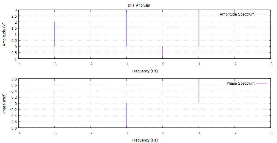
set multiplot layout 2,1 title "DFT Analysis"
set xlabel 'Frequency (Hz)'
set ylabel 'Amplitude (V)'
set grid
plot 'amplitude_spectrum.dat' with impulses title 'Amplitude Spectrum'

set xlabel 'Frequency (Hz)'
set ylabel 'Phase (rad)'
set grid
plot 'phase_spectrum.dat' with impulses title 'Phase Spectrum'
unset multiplot
set terminal png
set output 'amplitude_spectrum.png'
set xlabel 'Frequency (Hz)'
set ylabel 'Amplitude (V)'
set grid
plot 'amplitude_spectrum.dat' with impulses title 'Amplitude Spectrum'
set output
quit