A measure of similarity#
A method to determine the similarity between two real discrete signals, \( x \) and \( y \), involves multiplying each pair of corresponding samples from the signals and then summing the products.
Let's work through an example:
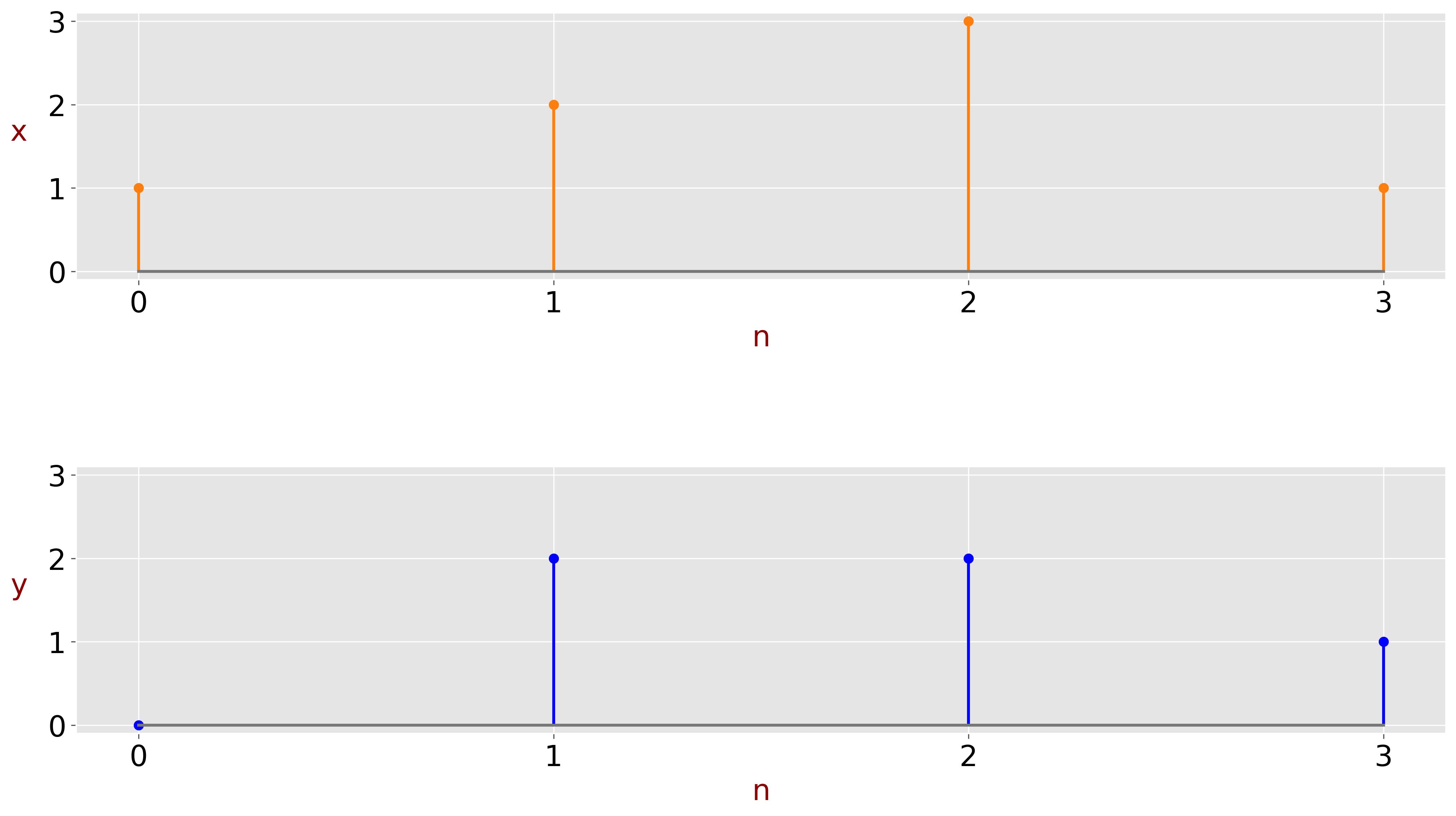
Consider the following sampled signals:
\( x = [1,2,3,1] \)
\( y = [0,2,2,1] \)

-
Multiply each pair of corresponding samples:
\( 1 \times 0 = 0 \)
\( 2 \times 2 = 4 \)
\( 3 \times 2 = 6 \)
\( 1 \times 1 = 1 \)
-
Sum the results of these multiplications:
\( r_{xy} = 0 + 4 + 6 + 1 = 11 \)
In signal processing terminology, the measure of similarity is often referred to as correlation, although this differs from the statistical definition of correlation.
Interpreting the Results#
A positive correlation signifies a positive similarity between the two signals, meaning they tend to increase or decrease together. A negative correlation indicates an inverse relationship, where one signal increases while the other decreases. Zero correlation suggests that the two signals are independent of each other. Such signals are referred to as uncorrelated or orthogonal signals.
Orthogonality is a fundamental concept in signal processing and many areas of mathematics and engineering, particularly in Fourier analysis and vector spaces. We will delve deeper into the topic of orthogonality later in this chapter.
Normalization#
To obtain a more meaningful measure of similarity, the result should be normalized. The normalized measure of similarity or correlation score for two real signals is given by:
\[ c_{xy} = \frac{r_{xy}}{\sqrt{r_{xx}} \sqrt{r_{yy}}} = \frac{\sum\limits_{n=-\infty}^{\infty} x_n y_n}{\sqrt{\sum\limits_{k=-\infty}^{\infty} x_n^2} \sqrt{\sum\limits_{k=-\infty}^{\infty} y_n^2}} \]
The correlation score satisfies:
\[ -1 \leq c_{xy} \leq 1 \]
This normalized measure provides a more accurate reflection of the similarity between the two signals.
In signal processing, the correlation score indicates the similarity between signals: a score close to 1 signifies high similarity, a score close to -1 indicates high inverse similarity, and a score close to 0 suggests low dependency between the signals.
In our example, the measure of similarity between the two signals is very high:
\[ c_{xy} = \frac{1 \times 0 + 2 \times 2 + 3 \times 2 + 1 \times 1}{\sqrt{1^2 + 2^2 + 3^2 + 1^2} \sqrt{0^2 + 2^2 + 2^2 + 1^2}} = \frac{11}{11.62} = 0.95 \]
Geometrical Interpretation#
We can represent signals \( x \) and \( y \) as vectors \( \mathbf{x} \) and \( \mathbf{y} \) respectively. In our example, each vector has four elements, meaning they exist in a four-dimensional space.
\[ \mathbf{x} = \begin{bmatrix} 1 \\ 2 \\ 3 \\ 1 \end{bmatrix}, \quad \mathbf{y} = \begin{bmatrix} 0 \\ 2 \\ 2 \\ 1 \end{bmatrix} \]
While we can draw and visualize vectors in two or three dimensions, visualizing them in higher dimensions is impossible.
In vector notation, the normalized measure of similarity between two vectors is often expressed using the vectors' dot product normalized by their magnitudes (norms):
\[ c_{xy} = \frac{\mathbf{x} \cdot \mathbf{y}}{\|\mathbf{x}\| \|\mathbf{y}\|} = \cos(\theta) \]
The normalized measure of similarity between two vectors \( \mathbf{x} \) and \( \mathbf{y} \) is defined as the cosine of the angle between them. This measure is often called cosine similarity.
Dot product reminder:
The dot product of two vectors \( \mathbf{x} \) and \( \mathbf{y} \) is defined as:
\[ \mathbf{x} \cdot \mathbf{y} = \|\mathbf{x}\| \|\mathbf{y}\| \cos(\theta) = \sum\limits_{n=-\infty}^{\infty} x_n y_n \]
Where:
- \( \theta \) is the angle between vectors.
- \( \|\mathbf{x}\| \) and \( \|\mathbf{y}\| \) are the Euclidean norms (magnitudes) of the vectors \( \mathbf{x} \) and \( \mathbf{y} \), respectively.
The Euclidean norm of a vector \( \mathbf{x} \) is given by:
\[ \|\mathbf{x}\| = \sqrt{\sum\limits_{n=-\infty}^{\infty} x_n^2} \]
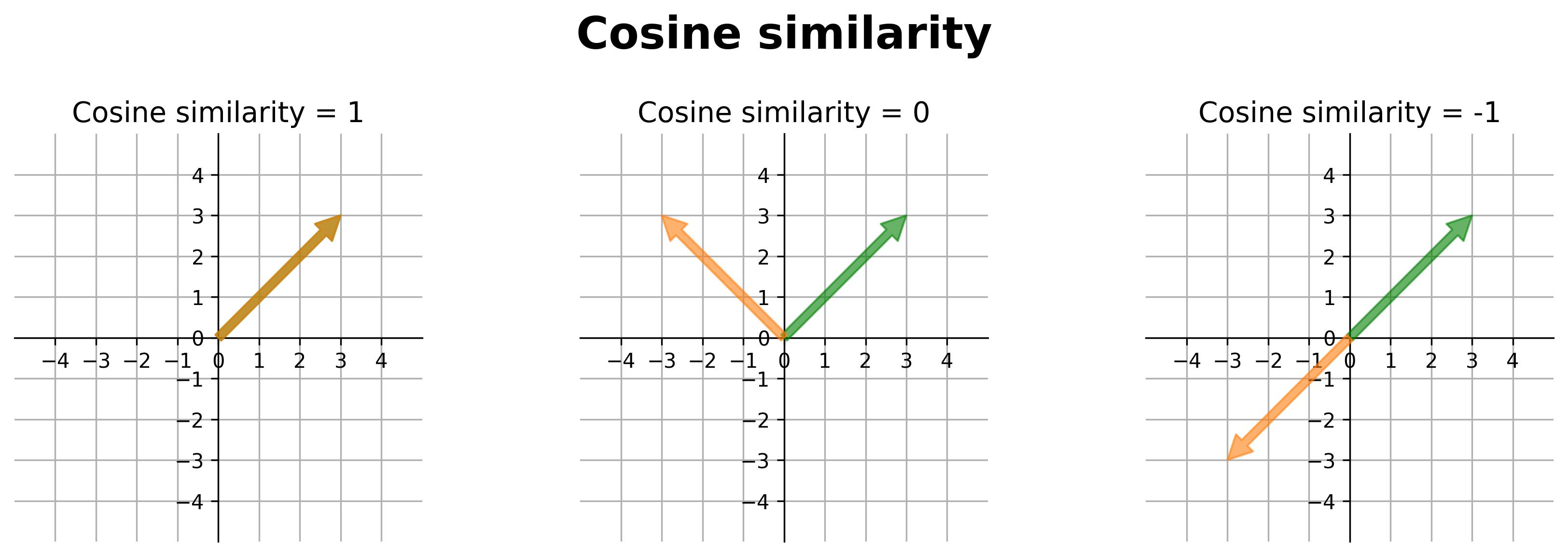
- When the vectors point in the same direction, the angle between them is zero, making \( \cos(\theta) = 1 \).
- When the vectors point in opposite directions, the angle between them is \( \pi \), making \( \cos(\theta) = -1 \).
- When the vectors are orthogonal (perpendicular), the angle between them is \( \pi /2 \), making \( \cos(\theta) = 0 \).
In vector notation, the dot product can be expressed as the product of the transpose of one vector with the other vector:
\[ \mathbf{x} \cdot \mathbf{y} = \mathbf{x}^T \mathbf{y} = \mathbf{y}^T \mathbf{x} \]
In our example:
\[ \mathbf{x} \cdot \mathbf{y} = \mathbf{x}^T \mathbf{y} = \begin{bmatrix} 1 & 2 & 3 & 1 \end{bmatrix} \begin{bmatrix} 0 \\ 2 \\ 2 \\ 1 \end{bmatrix} = 0 + 4 + 6 + 1 = 11 \]
The following figure exemplifies the cosine similarity for 2D vectors at different angles between vectors.

In reality, each signal has much more than two samples. You can imagine a sampled signal as a vector in a multi-dimensional space.