Orthogonality#
In geometry, vectors are considered orthogonal if they are perpendicular to each other, which is determined by their dot product being zero (i.e., the sum of the products of their corresponding elements equals zero).
\[ \mathbf{x} \cdot \mathbf{y} = \|\mathbf{x}\| \|\mathbf{y}\| \cos(\theta) = \sum\limits_{n=-\infty}^{\infty} x_n y_n = 0 \]
This means that the \( \theta \) between the vectors is \( 90^\circ \) (or \( \pi /2 \) radians), and the cosine of \( \theta \) is zero.
Consequently, the measure of similarity of two orthogonal discrete-time signals equals zero:
\[ c_{xy} = \frac{\mathbf{x} \cdot \mathbf{y}}{\|\mathbf{x}\| \|\mathbf{y}\|} = \frac{\sum\limits_{n=-\infty}^{\infty} x_n y_n}{\sqrt{\sum\limits_{k=-\infty}^{\infty} x_n^2} \sqrt{\sum\limits_{k=-\infty}^{\infty} y_n^2}} = 0 \]
Orthogonality in the context of functions extends the concept of orthogonality in vectors. For continuous functions, orthogonality is determined by an inner product, where the functions are treated as if they had infinitely many components. In the "continuous world," the sum operator becomes an integral. The inner product of two functions is found by multiplying the functions together and integrating the product over a given interval.
Two real non-zero functions \( f(x) \) and \( g(x) \) are said to be orthogonal on an interval \( a \leq x \leq b \) if their inner product on the interval equals zero:
\[ \langle f(x), g(x) \rangle = \int\limits_{a}^{b} f(x) g(x) \,dx = 0 \]
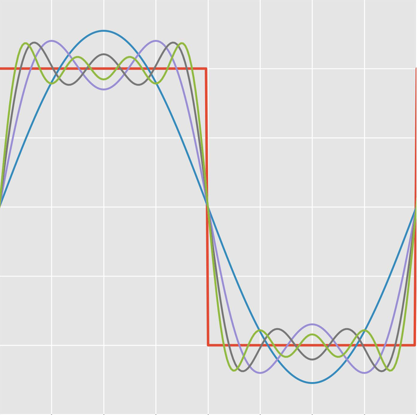
Sine and cosine are among the most well-known and widely used orthogonal functions. Their orthogonality plays a crucial role in various mathematical, engineering, and scientific applications, including Fourier analysis.
As we will see later, sine and cosine functions form the basis of the Fourier series, which decomposes periodic functions into sums of sines and cosines. This decomposition is essential for analyzing and synthesizing periodic signals.
To prove the orthogonality of sine and cosine functions, we must show that their inner product over one period is zero. This is typically done over the interval \([0,2\pi]\) or any interval of length \(2\pi\).
\[ \int\limits_{0}^{2\pi} \sin(\theta) \cos(\theta) \,d\theta \]
Let us use the trigonometric identity:
\[ \sin(\alpha) \cos(\beta) = \frac{1}{2} [\sin(\alpha - \beta) + \sin(\alpha + \beta)] \]
\[ \int\limits_{0}^{2\pi} \sin(\theta) \cos(\theta) \,d\theta = \frac{1}{2} \int\limits_{0}^{2\pi} \sin(2\theta) \,d\theta = -\frac{1}{4} [\cos(2\theta)]_{0}^{2\pi} \]
\[ = -\frac{1}{4} (\cos(4\pi) - \cos(0)) = 0 \]
Let us work through examples with sampled (discrete) sine and cosine functions.
Assume sine and cosine functions sampled at \( 2\pi /3 \) (120°) intervals.
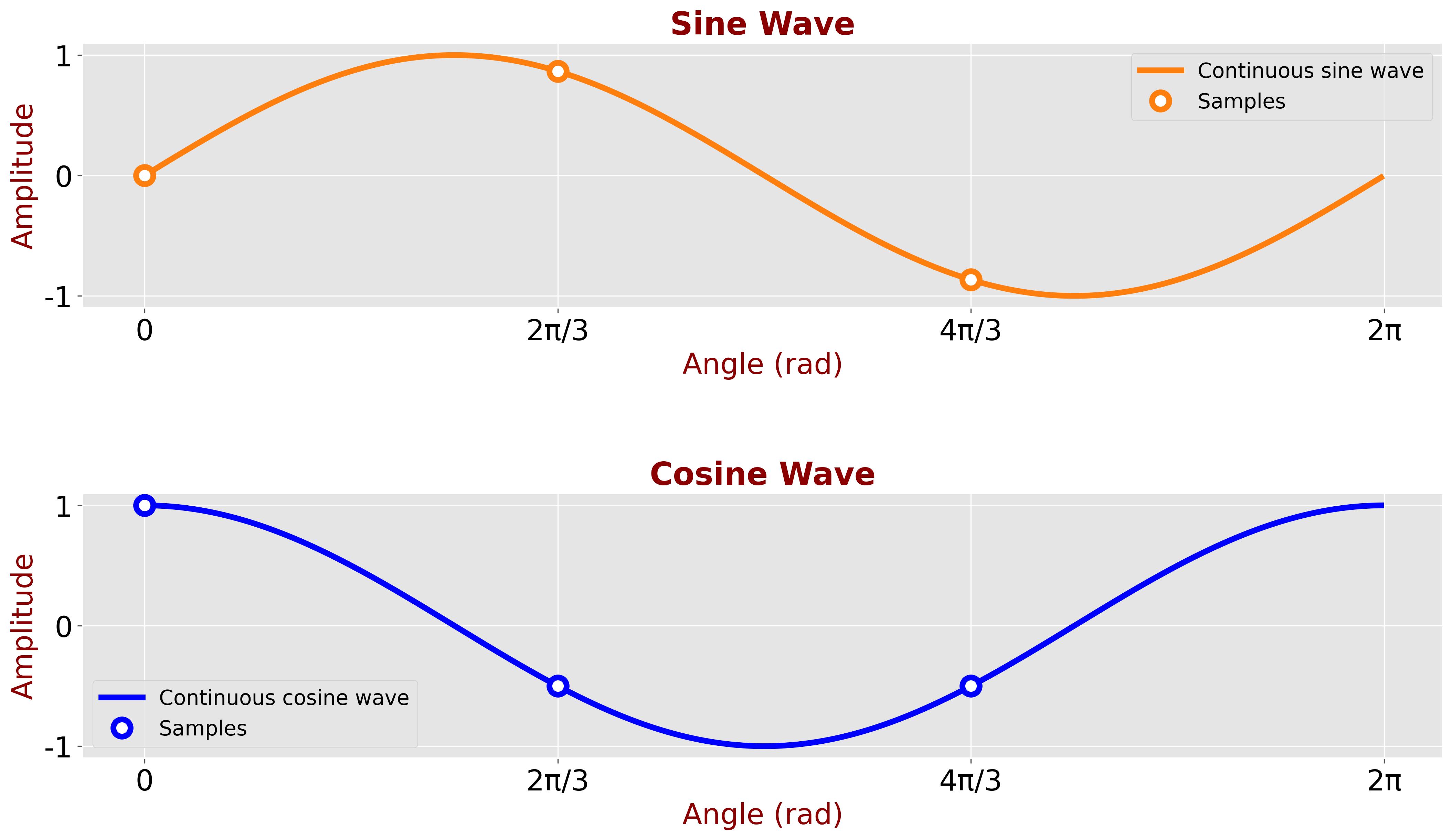
The table below shows the sampled values:
| n | Angle (\(\theta\)) | \(\sin(\theta)\) | \(\cos(\theta)\) | \(\sin(\theta) \cos(\theta)\) |
|---|---|---|---|---|
| 0 | \( \displaystyle 0 \) | \( \displaystyle 0 \) | \( \displaystyle 1 \) | \( \displaystyle 0 \) |
| 1 | \( \displaystyle \frac{2\pi}{3} \) | \( \displaystyle \frac{\sqrt{3}}{2} \) | \( \displaystyle -\frac{1}{2} \) | \( \displaystyle -\frac{\sqrt{3}}{4} \) |
| 2 | \( \displaystyle \frac{4\pi}{3} \) | \( \displaystyle -\frac{\sqrt{3}}{2} \) | \( \displaystyle -\frac{1}{2} \) | \( \displaystyle \frac{\sqrt{3}}{4} \) |
In the discrete domain, the integral becomes a summation.
\[ \sum\limits_{n=0}^{2} \sin(\theta_n) \cos(\theta_n) = 0 - \frac{\sqrt{3}}{4} + \frac{\sqrt{3}}{4} = 0 \]
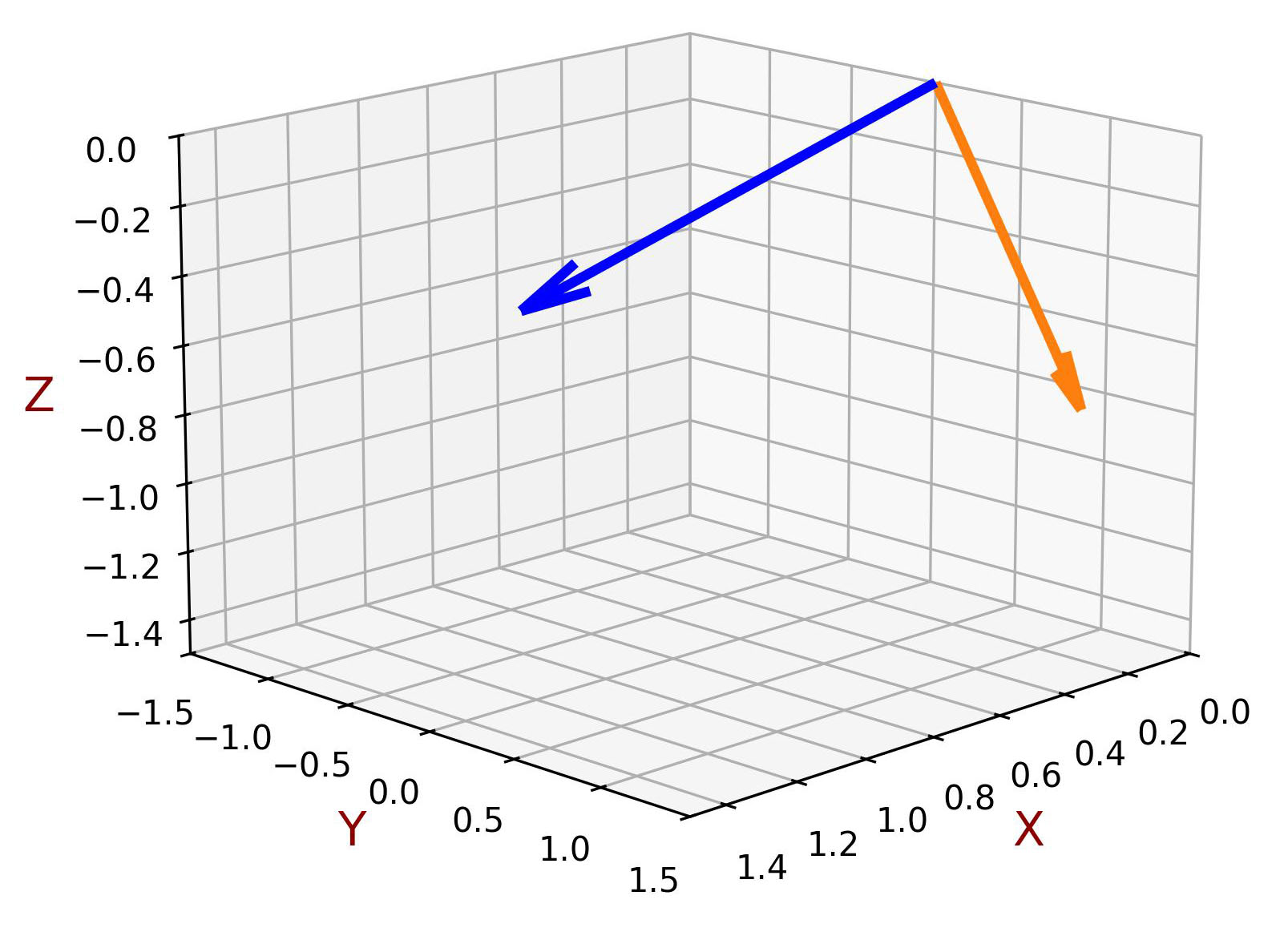
Geometric Interpretation
In this example, the sine and cosine functions are sampled at three equally spaced points, resulting in two 3-dimensional vectors:
\[ \sin(\theta) = \begin{bmatrix} 0 \\ \displaystyle \frac{\sqrt{3}}{2} \\ \displaystyle -\frac{\sqrt{3}}{2} \end{bmatrix}, \quad \cos(\theta) = \begin{bmatrix} \displaystyle 1 \\ \displaystyle -\frac{1}{2} \\ \displaystyle -\frac{1}{2} \end{bmatrix} \]
As shown in the figure, the angle between these two vectors is \( 90^\circ \) (or \( \pi /2 \) radians), indicating that the sine and cosine vectors are orthogonal.
Now, let’s increase the sampling rate to 8 samples per period.
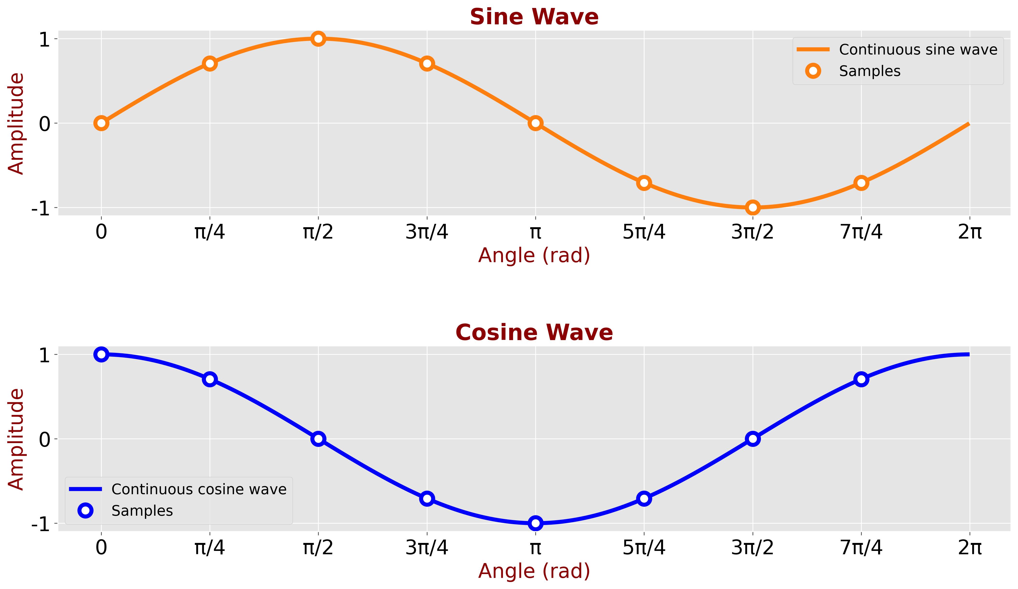
The table below shows the sampled values:
| n | Angle (\(\theta\)) | \(\sin(\theta)\) | \(\cos(\theta)\) | \(\sin(\theta) \cos(\theta)\) |
|---|---|---|---|---|
| 0 | \(\displaystyle 0 \) | \(\displaystyle 0 \) | \(\displaystyle 1 \) | \(\displaystyle 0 \) |
| 1 | \(\displaystyle \frac{\pi}{4} \) | \(\displaystyle \frac{1}{\sqrt{2}} \) | \(\displaystyle \frac{1}{\sqrt{2}} \) | \(\displaystyle \frac{1}{2} \) |
| 2 | \(\displaystyle \frac{\pi}{2} \) | \(\displaystyle 1 \) | \(\displaystyle 0 \) | \(\displaystyle 0 \) |
| 3 | \(\displaystyle \frac{3\pi}{4} \) | \(\displaystyle \frac{1}{\sqrt{2}} \) | \(\displaystyle -\frac{1}{\sqrt{2}} \) | \(\displaystyle -\frac{1}{2} \) |
| 4 | \(\displaystyle \pi \) | \(\displaystyle 0 \) | \(\displaystyle -1 \) | \(\displaystyle 0 \) |
| 5 | \(\displaystyle \frac{5\pi}{4} \) | \(\displaystyle -\frac{1}{\sqrt{2}} \) | \(\displaystyle -\frac{1}{\sqrt{2}} \) | \(\displaystyle \frac{1}{2} \) |
| 6 | \(\displaystyle \frac{3\pi}{2} \) | \(\displaystyle -1 \) | \(\displaystyle 0 \) | \(\displaystyle 0 \) |
| 7 | \(\displaystyle \frac{7\pi}{4} \) | \(\displaystyle -\frac{1}{\sqrt{2}} \) | \(\displaystyle \frac{1}{\sqrt{2}} \) | \(\displaystyle -\frac{1}{2} \) |
The dot product is:
\[ \sum\limits_{n=0}^{7} \sin(\theta_n) \cos(\theta_n) = 0 + \frac{1}{2} + 0 - \frac{1}{2} + 0 + \frac{1}{2} + 0 - \frac{1}{2} = 0 \]
As observed, the sine and cosine functions remain orthogonal even with increased sampling density.
Geometric Interpretation
In this example, the sine and cosine functions are sampled at eight equally spaced points, producing two 8-dimensional vectors:
\[ \sin(\theta) = \begin{bmatrix} 0 \\ \displaystyle \frac{1}{\sqrt{2}} \\ \displaystyle 1 \\ \displaystyle \frac{1}{\sqrt{2}} \\ 0 \\ \displaystyle -\frac{1}{\sqrt{2}} \\ \displaystyle -1 \\ \displaystyle -\frac{1}{\sqrt{2}} \end{bmatrix}, \quad \cos(\theta) = \begin{bmatrix} \displaystyle 1 \\ \displaystyle \frac{1}{\sqrt{2}} \\ \displaystyle 0 \\ \displaystyle -\frac{1}{\sqrt{2}} \\ \displaystyle -1 \\ \displaystyle -\frac{1}{\sqrt{2}} \\ \displaystyle 0 \\ \displaystyle \frac{1}{\sqrt{2}} \end{bmatrix} \]
These vectors, although hard to visualize due to their 8-dimensional nature, can be mathematically analyzed. The key point is that in the space defined by these eight dimensions, the angle between these vectors is \( 90^\circ \) (or \( \pi /2 \) radians). This implies that the sine and cosine vectors are orthogonal.
This example illustrates how mathematical abstraction extends beyond our physical intuition, enabling us to analyze properties in higher-dimensional spaces. The concept of multiplying two vectors and obtaining a zero result is generalized in mathematics as orthogonality.
Orthogonal Functions in Fourier Transform#
The following functions are integral expressions that demonstrate the orthogonality of sine and cosine functions over a period \( T \).
\[ \int\limits_0^T \sin(m\omega t) \cos(n\omega t) \,dt = 0 \]
\[ \int\limits_0^T \sin(m\omega t) \sin(n\omega t) \,dt = \begin{cases} 0 & m \neq n \\ \frac{T}{2} & m = n \end{cases} \]
\[ \int\limits_0^T \cos(m\omega t) \cos(n\omega t) \,dt = \begin{cases} 0 & m \neq n \\ \frac{T}{2} & m = n \end{cases} \]
Where \( m \) and \( n \) are integers.
The derivations for the above integrals are provided in Appendix B.
The integrals show that sine and cosine functions of different frequencies (\( m\omega \) and \( n\omega \)) are orthogonal, meaning their integrals over one period \( T \) are zero. This orthogonality is key to isolating individual frequency components in a signal when performing a Fourier transform.
On the other hand, the integrals for \( m=n \) provide the energy of the sine and cosine functions over a period \( T \). This allows the Fourier transform to precisely quantify the contribution of each frequency to the signal's total energy.
These orthogonal relationships are fundamental to the Fourier transform.
Other orthogonal functions#
Orthogonal functions are essential in many areas of science and engineering due to their unique properties and applications.
In communication systems, orthogonal codes are utilized in the Code-Division Multiple Access (CDMA) technique, allowing multiple signals to share the same channel or frequency band without causing mutual interference.
Orthogonal Frequency Division Multiplexing (OFDM) is another communication technique that leverages orthogonality. OFDM uses closely spaced orthogonal sub-carrier signals to carry data. The orthogonality ensures that even though the sub-carriers overlap in the frequency domain, they have no mutual interference. This allows for efficient use of the available spectrum.