DFT Example:
Input signal parameters extraction.
Important note!
In the following example, I use carefully chosen signals and sample rate to illustrate key concepts clearly. Changing the sample rate will produce different results, which require further explanation. I will address this in later sections.
The input signal#
Assume an arbitrary input signal:
\[ x(t) = \sum_{m=1}^{M} A_m \sin\left( \omega_m t + \phi_m \right) \]
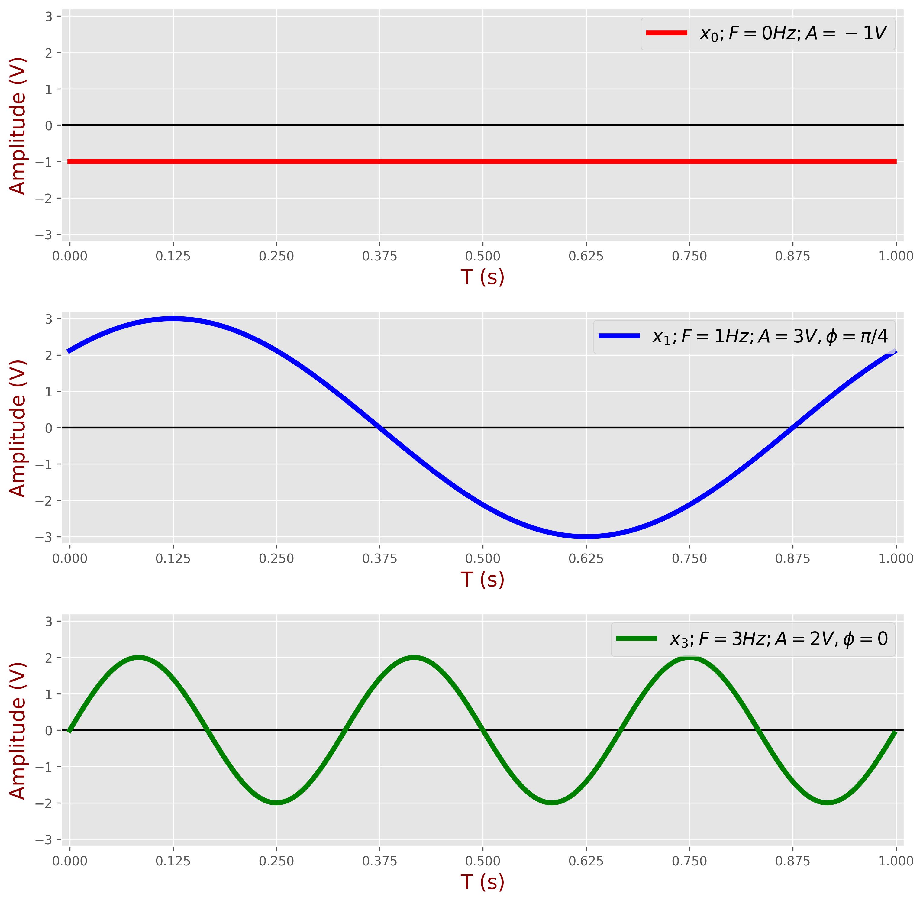
The input signal includes the following three components:
- DC: \( A = -1V \), \( f = 0 \text{Hz} \)
- 1Hz component: \( A = 3V \), \( f = 1\text{Hz} \), \( \phi = \pi/4 \)
- 3Hz component: \( A = 2V \), \( f = 3\text{Hz} \), \( \phi = 0 \)
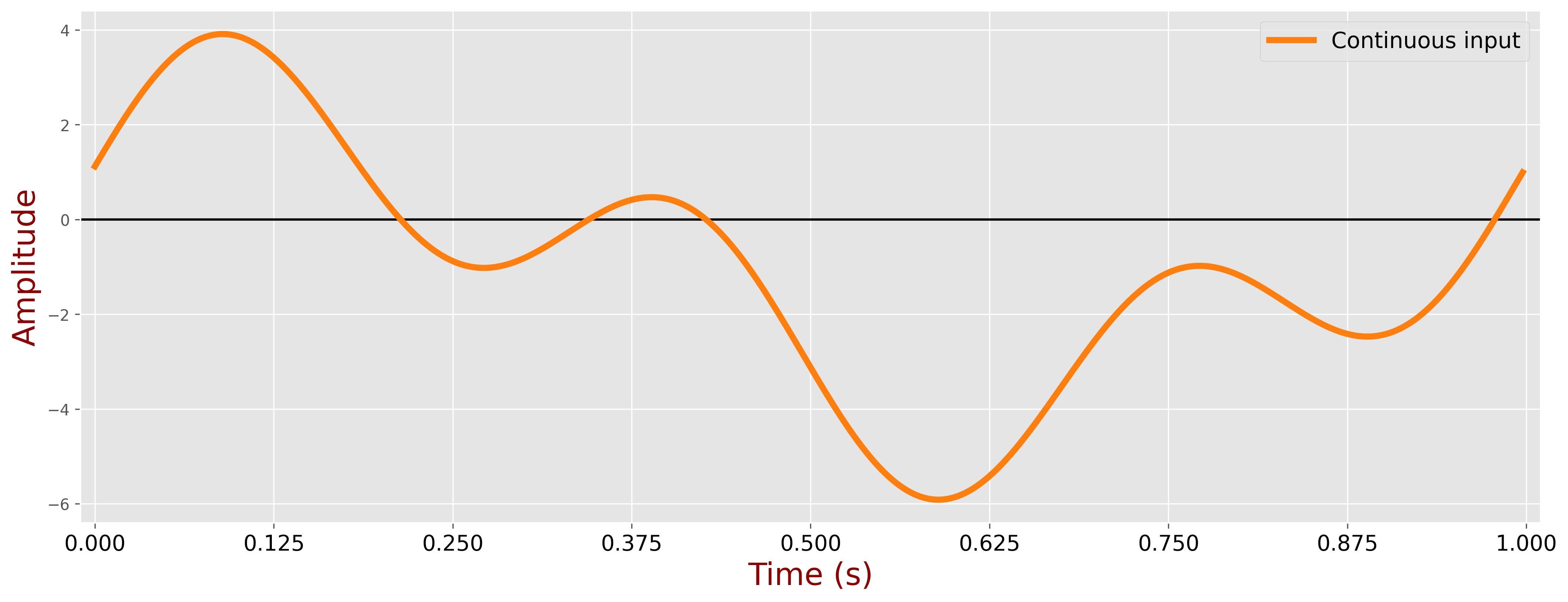
The input signal can be expressed as:
\[ x_{\text{in}}(t) = -1 + 3\sin\left(2\pi \cdot 1 \cdot t + \frac{\pi}{4}\right) + 2\sin\left(2\pi \cdot 3 \cdot t\right) \]
The following plot illustrates the three components of the input signal:
The subsequent plot depicts the input signal as the sum of these three components:
The input signal is sampled by an ADC with a sampling frequency of \( f_s = 8\text{Hz} \) during a period of 1 second (\( T = 1\text{s} \)), resulting in 8 samples:
\[ N = T f_s = 8 \]
The sampling period is:
\[ t_s = \frac{1}{f_s} = \frac{1}{8} = 0.125\text{s} \]
Meaning samples are taken every 0.125 seconds.
The sampled signal can be expressed as:
\[ x_{\text{in}}[n] = \sum_{m=1}^{M} A_m \sin\left(2\pi f t_s n + \phi_m\right) \]
\[ = -1 + 3\sin\left(2\pi \cdot \frac{1}{8} n + \frac{\pi}{4}\right) + 2\sin\left(2\pi \cdot 3 \cdot \frac{1}{8} n\right) \]
The following plot illustrates the sampled input signal:
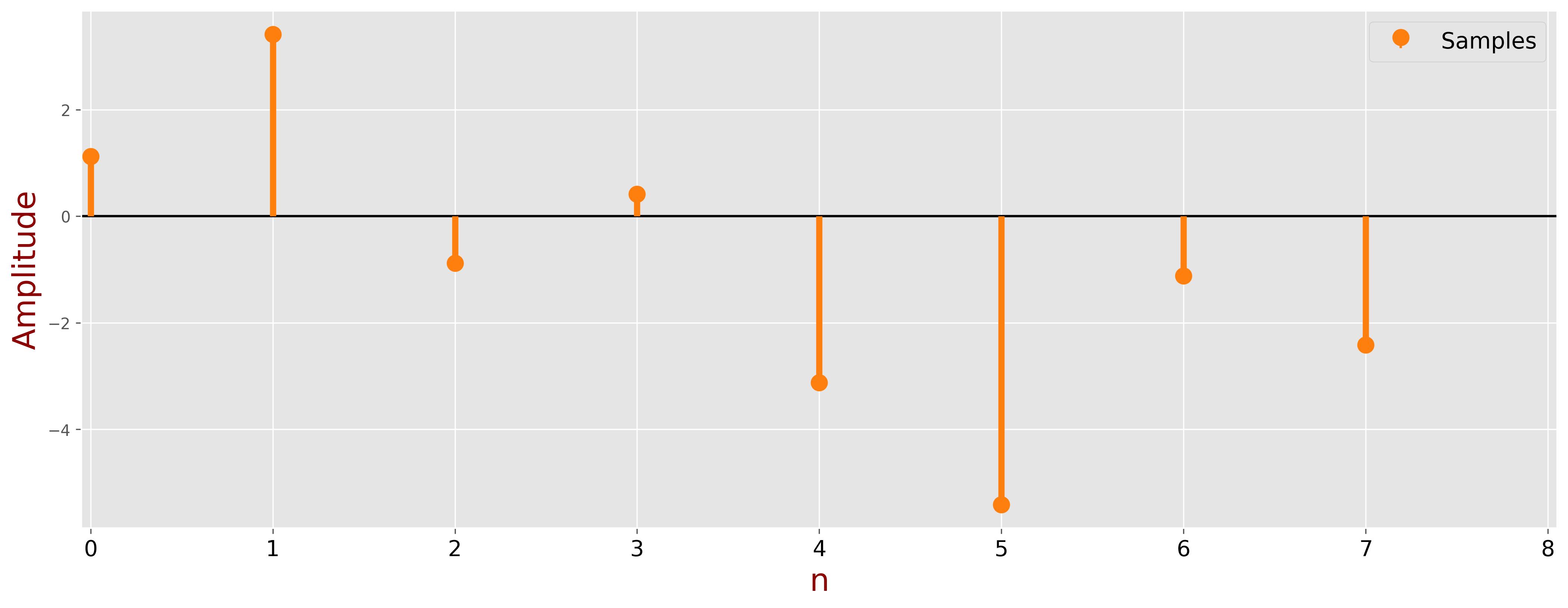
The table below presents the sample values of each component of the input signal (DC, 1Hz, and 3Hz) and their sum. The samples are calculated at specific time instances, illustrating how the individual components combine to form the overall input signal.
| \( n \) | 0 | 1 | 2 | 3 | 4 | 5 | 6 | 7 |
|---|---|---|---|---|---|---|---|---|
| \( x_0[n] \) | -1 | -1 | -1 | -1 | -1 | -1 | -1 | -1 |
| \( x_1[n] \) | \( \frac{3}{\sqrt{2}} \) | 3 | \( \frac{3}{\sqrt{2}} \) | 0 | \( -\frac{3}{\sqrt{2}} \) | -3 | \( -\frac{3}{\sqrt{2}} \) | 0 |
| \( x_3[n] \) | 0 | \( \frac{2}{\sqrt{2}} \) | -2 | \( \frac{2}{\sqrt{2}} \) | 0 | \( -\frac{2}{\sqrt{2}} \) | 2 | \( -\frac{2}{\sqrt{2}} \) |
| \( x_{\text{in}}[n] \) | \( \frac{3-\sqrt{2}}{\sqrt{2}} \) | \( \frac{2+2\sqrt{2}}{\sqrt{2}} \) | \( \frac{3-3\sqrt{2}}{\sqrt{2}} \) | \( \frac{2-\sqrt{2}}{\sqrt{2}} \) | \( \frac{-3-\sqrt{2}}{\sqrt{2}} \) | \( \frac{-2-4\sqrt{2}}{\sqrt{2}} \) | \( \frac{-3+\sqrt{2}}{\sqrt{2}} \) | \( \frac{-2-\sqrt{2}}{\sqrt{2}} \) |
The predefined sine-cosine pairs#
In the previous chapter, we derived the range for discrete frequencies \( f_k \):
\[ 0 \leq k \leq N - 1 \]
The periodic sine wave with frequency \( f_k \) is expressed as:
\[ x_s[n] = \sin\left( \frac{2\pi k}{N} n \right) \]
Similarly, the periodic cosine wave with frequency \( f_k \) is:
\[ x_c[n] = \cos\left( \frac{2\pi k}{N} n \right) \]
The relation between the discrete frequencies and corresponding analog frequencies is given by:
\[ f = \begin{cases} \dfrac{k}{N} f_s, & 0 \leq k \leq \dfrac{N}{2} - 1 \\ \\ \dfrac{k - N}{N} f_s, & \dfrac{N}{2} \leq k \leq N - 1 \end{cases} \]
The following table describes the relation between \(k\) and analog frequencies:
| \( k \) | Analog Frequency |
|---|---|
| 0 | \( -\dfrac{0}{8} f_s = 0\text{Hz} \) |
| 1 | \( \dfrac{1}{8} f_s = 1\text{Hz} \) |
| 2 | \( \dfrac{2}{8} f_s = 2\text{Hz} \) |
| 3 | \( \dfrac{3}{8} f_s = 3\text{Hz} \) |
| 4 | \( -\dfrac{4}{8} f_s = -4\text{Hz} \) |
| 5 | \( -\dfrac{3}{8} f_s = -3\text{Hz} \) |
| 6 | \( -\dfrac{2}{8} f_s = -2\text{Hz} \) |
| 7 | \( -\dfrac{1}{8} f_s = -1\text{Hz} \) |
The plot below shows sampled sine and cosine functions, with red markers indicating the sampled points.
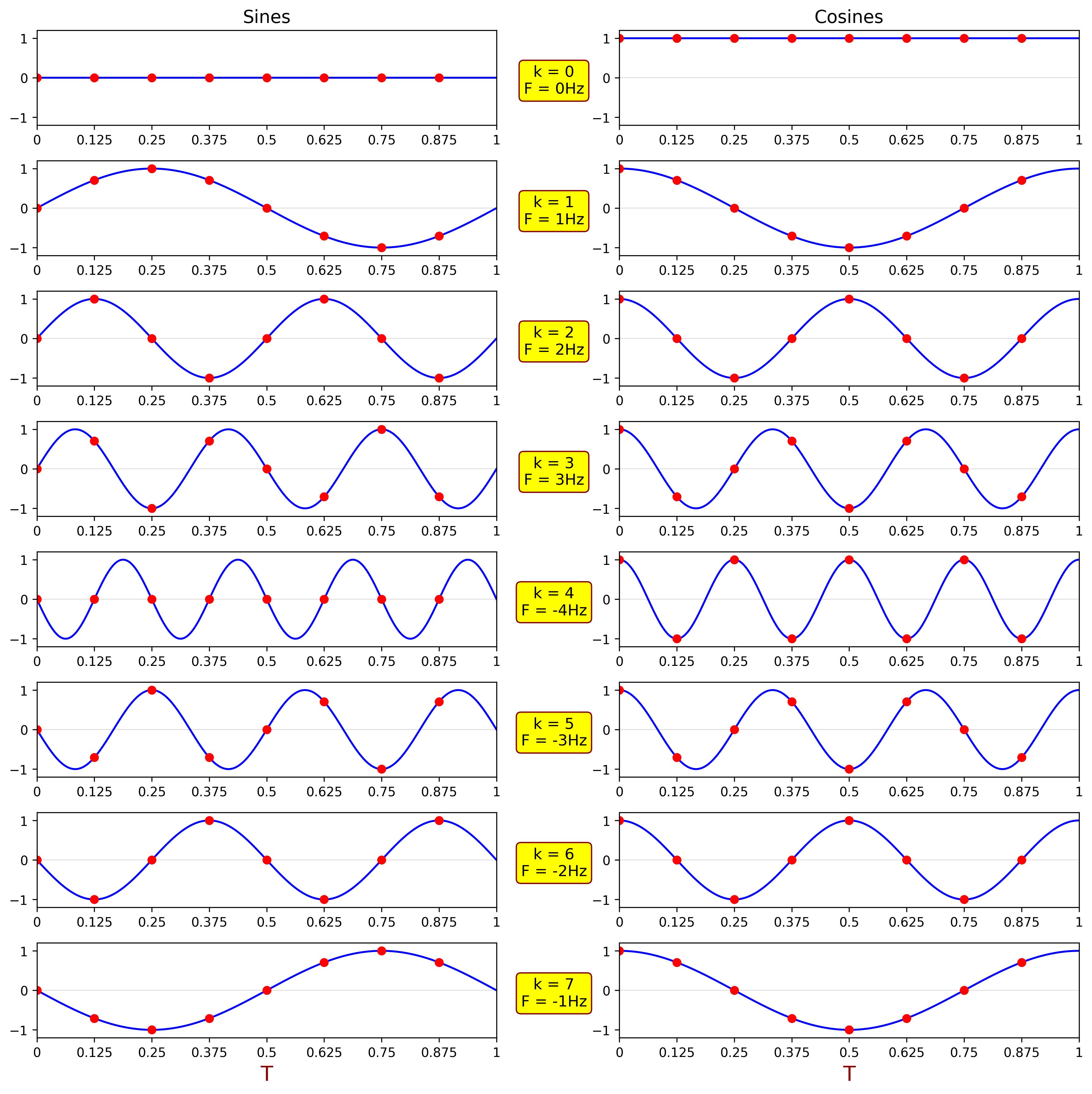
Note that cosine values are identical for both positive and negative frequencies because cosine is an even function: \( \cos(-\alpha) = \cos(\alpha) \). In contrast, sine values are negated for positive and negative frequencies because sine is an odd function: \( \sin(-\alpha) = -\sin(\alpha) \).
The table below displays the sample values of the predefined sine and cosine function samples. These values are used to compute the correlation with the input signal.
| \( k \) (Frequency) |
Function | 0 | 1 | 2 | 3 | 4 | 5 | 6 | 7 |
|---|---|---|---|---|---|---|---|---|---|
| \(k = 0\) \((f = 0\text{Hz})\) |
\( \sin(0) \) | 0 | 0 | 0 | 0 | 0 | 0 | 0 | 0 |
| \( \cos(0) \) | 1 | 1 | 1 | 1 | 1 | 1 | 1 | 1 | |
| \(k = 1\) \((f = 1\text{Hz})\) |
\( \sin\left(2\pi \frac{1}{8} n\right) \) | 0 | \( \frac{1}{\sqrt{2}} \) | 1 | \( \frac{1}{\sqrt{2}} \) | 0 | \( -\frac{1}{\sqrt{2}} \) | -1 | \( -\frac{1}{\sqrt{2}} \) |
| \( \cos\left(2\pi \frac{1}{8} n\right) \) | 1 | \( \frac{1}{\sqrt{2}} \) | 0 | \( -\frac{1}{\sqrt{2}} \) | -1 | \( -\frac{1}{\sqrt{2}} \) | 0 | \( \frac{1}{\sqrt{2}} \) | |
| \(k = 2\) \((f = 2\text{Hz})\) |
\( \sin\left(2\pi \frac{2}{8} n\right) \) | 0 | 1 | 0 | -1 | 0 | 1 | 0 | -1 |
| \( \cos\left(2\pi \frac{2}{8} n\right) \) | 1 | 0 | -1 | 0 | 1 | 0 | -1 | 0 | |
| \(k = 3\) \((f = 3\text{Hz})\) |
\( \sin\left(2\pi \frac{3}{8} n\right) \) | 0 | \( \frac{1}{\sqrt{2}} \) | -1 | \( \frac{1}{\sqrt{2}} \) | 0 | \( -\frac{1}{\sqrt{2}} \) | 1 | \( -\frac{1}{\sqrt{2}} \) |
| \( \cos\left(2\pi \frac{3}{8} n\right) \) | 1 | \( -\frac{1}{\sqrt{2}} \) | 0 | \( \frac{1}{\sqrt{2}} \) | -1 | \( \frac{1}{\sqrt{2}} \) | 0 | \( -\frac{1}{\sqrt{2}} \) | |
| \(k = 4\) \((f = -4\text{Hz})\) |
\( \sin\left(2\pi \frac{4}{8} n\right) \) | 0 | 0 | 0 | 0 | 0 | 0 | 0 | 0 |
| \( \cos\left(2\pi \frac{4}{8} n\right) \) | 1 | -1 | 1 | -1 | 1 | -1 | 1 | -1 | |
| \(k = 5\) \((f = -3\text{Hz})\) |
\( \sin\left(2\pi \frac{5}{8} n\right) \) | 0 | \( -\frac{1}{\sqrt{2}} \) | 1 | \( -\frac{1}{\sqrt{2}} \) | 0 | \( \frac{1}{\sqrt{2}} \) | -1 | \(\frac{1}{\sqrt{2}} \) |
| \( \cos\left(2\pi \frac{5}{8} n\right) \) | 1 | \( -\frac{1}{\sqrt{2}} \) | 0 | \( \frac{1}{\sqrt{2}} \) | -1 | \( \frac{1}{\sqrt{2}} \) | 0 | \( -\frac{1}{\sqrt{2}} \) | |
| \(k = 6\) \((f = -2\text{Hz})\) |
\( \sin\left(2\pi \frac{6}{8} n\right) \) | 0 | -1 | 0 | 1 | 0 | -1 | 0 | 1 |
| \( \cos\left(2\pi \frac{6}{8} n\right) \) | 1 | 0 | -1 | 0 | 1 | 0 | -1 | 0 | |
| \(k = 7\) \((f = -1\text{Hz})\) |
\( \sin\left(2\pi \frac{7}{8} n\right) \) | 0 | \( -\frac{1}{\sqrt{2}} \) | -1 | \( -\frac{1}{\sqrt{2}} \) | 0 | \( \frac{1}{\sqrt{2}} \) | 1 | \( \frac{1}{\sqrt{2}} \) |
| \( \cos\left(2\pi \frac{7}{8} n\right) \) | 1 | \( \frac{1}{\sqrt{2}} \) | 0 | \( -\frac{1}{\sqrt{2}} \) | -1 | \( -\frac{1}{\sqrt{2}} \) | 0 | \( \frac{1}{\sqrt{2}} \) |
DFT coefficients computation#
We aim to calculate the correlation between the input signal and predefined sine-cosine pairs. This analysis will help identify the presence and contribution of specific frequency components within the input signal.
First, let’s define the DFT coefficients. The cosine-weighted coefficients are given by:
\[ a_k = \frac{2}{N} \sum_{n=0}^{N-1} x(n) \cos\left( \frac{2\pi k}{N} n \right) \]
\[ \begin{aligned} a_0 &= \frac{2}{8} \left( \frac{3-\sqrt{2}}{\sqrt{2}} + \frac{2+2\sqrt{2}}{\sqrt{2}} + \frac{3-3\sqrt{2}}{\sqrt{2}} + \frac{2-\sqrt{2}}{\sqrt{2}} + \frac{-3-\sqrt{2}}{\sqrt{2}} + \frac{-2-4\sqrt{2}}{\sqrt{2}} + \frac{-3+\sqrt{2}}{\sqrt{2}} + \frac{-2-\sqrt{2}}{\sqrt{2}} \right) = -2 \\ a_1 &= \frac{2}{8} \left( \frac{3-\sqrt{2}}{\sqrt{2}} \cdot 1 + \frac{2+2\sqrt{2}}{\sqrt{2}} \cdot \frac{1}{\sqrt{2}} + \frac{3-3\sqrt{2}}{\sqrt{2}} \cdot 0 + \frac{2-\sqrt{2}}{\sqrt{2}} \cdot \frac{-1}{\sqrt{2}} + \frac{-3-\sqrt{2}}{\sqrt{2}} \cdot (-1) + \frac{-2-4\sqrt{2}}{\sqrt{2}} \cdot \frac{-1}{\sqrt{2}} + \frac{-3+\sqrt{2}}{\sqrt{2}} \cdot 0 + \frac{-2-\sqrt{2}}{\sqrt{2}} \cdot \frac{1}{\sqrt{2}} \right) = \frac{3}{2}\sqrt{2} \\ a_2 &= \frac{2}{8} \left( \frac{3-\sqrt{2}}{\sqrt{2}} \cdot 1 + \frac{2+2\sqrt{2}}{\sqrt{2}} \cdot 0 + \frac{3-3\sqrt{2}}{\sqrt{2}} \cdot (-1) + \frac{2-\sqrt{2}}{\sqrt{2}} \cdot 0 + \frac{-3-\sqrt{2}}{\sqrt{2}} \cdot 1 + \frac{-2-4\sqrt{2}}{\sqrt{2}} \cdot 0 + \frac{-3+\sqrt{2}}{\sqrt{2}} \cdot (-1) + \frac{-2-\sqrt{2}}{\sqrt{2}} \cdot 0 \right) = 0 \\ a_3 &= \frac{2}{8} \left( \frac{3-\sqrt{2}}{\sqrt{2}} \cdot 1 + \frac{2+2\sqrt{2}}{\sqrt{2}} \cdot \frac{-1}{\sqrt{2}} + \frac{3-3\sqrt{2}}{\sqrt{2}} \cdot 0 + \frac{2-\sqrt{2}}{\sqrt{2}} \cdot \frac{1}{\sqrt{2}} + \frac{-3-\sqrt{2}}{\sqrt{2}} \cdot (-1) + \frac{-2-4\sqrt{2}}{\sqrt{2}} \cdot \frac{1}{\sqrt{2}} + \frac{-3+\sqrt{2}}{\sqrt{2}} \cdot 0 + \frac{-2-\sqrt{2}}{\sqrt{2}} \cdot \frac{-1}{\sqrt{2}} \right) = 0 \\ a_4 &= \frac{2}{8} \left( \frac{3-\sqrt{2}}{\sqrt{2}} \cdot 0 + \frac{2+2\sqrt{2}}{\sqrt{2}} \cdot 0 + \frac{3-3\sqrt{2}}{\sqrt{2}} \cdot 0 + \frac{2-\sqrt{2}}{\sqrt{2}} \cdot 0 + \frac{-3-\sqrt{2}}{\sqrt{2}} \cdot 0 + \frac{-2-4\sqrt{2}}{\sqrt{2}} \cdot 0 + \frac{-3+\sqrt{2}}{\sqrt{2}} \cdot 0 + \frac{-2-\sqrt{2}}{\sqrt{2}} \cdot 0 \right) = 0 \end{aligned} \]
Cosine values are identical for both positive and negative frequencies:
\[ a_5 = a_3 = 0, \quad a_6 = a_2 = 0, \quad a_7 = a_1 = \frac{3}{2}\sqrt{2} \]
The sine-weighted coefficients are given by:
\[ b_k = \frac{2}{N} \sum_{n=0}^{N-1} x(n) \sin\left( \frac{2\pi k}{N} n \right) \]
\[ \begin{aligned} b_0 &= \frac{2}{8} \left( \frac{3-\sqrt{2}}{\sqrt{2}} \cdot 0 + \frac{2+2\sqrt{2}}{\sqrt{2}} \cdot 0 + \frac{3-3\sqrt{2}}{\sqrt{2}} \cdot 0 + \frac{2-\sqrt{2}}{\sqrt{2}} \cdot 0 + \frac{-3-\sqrt{2}}{\sqrt{2}} \cdot 0 + \frac{-2-4\sqrt{2}}{\sqrt{2}} \cdot 0 + \frac{-3+\sqrt{2}}{\sqrt{2}} \cdot 0 + \frac{-2-\sqrt{2}}{\sqrt{2}} \cdot 0 \right) = 0 \\ b_1 &= \frac{2}{8} \left( 0 + \frac{2+2\sqrt{2}}{\sqrt{2}} \cdot \frac{1}{\sqrt{2}} + \frac{3-3\sqrt{2}}{\sqrt{2}} \cdot 1 + \frac{2-\sqrt{2}}{\sqrt{2}} \cdot \frac{1}{\sqrt{2}} + 0 + \frac{-2-4\sqrt{2}}{\sqrt{2}} \cdot \frac{-1}{\sqrt{2}} + \frac{-3+\sqrt{2}}{\sqrt{2}} \cdot (-1) + \frac{-2-\sqrt{2}}{\sqrt{2}} \cdot \frac{-1}{\sqrt{2}} \right) = \frac{3}{2}\sqrt{2} \\ b_2 &= \frac{2}{8} \left( \frac{3-\sqrt{2}}{\sqrt{2}} \cdot 0 + \frac{2+2\sqrt{2}}{\sqrt{2}} \cdot 1 + \frac{3-3\sqrt{2}}{\sqrt{2}} \cdot 0 + \frac{2-\sqrt{2}}{\sqrt{2}} \cdot (-1) + \frac{-3-\sqrt{2}}{\sqrt{2}} \cdot 0 + \frac{-2-4\sqrt{2}}{\sqrt{2}} \cdot 1 + \frac{-3+\sqrt{2}}{\sqrt{2}} \cdot 0 + \frac{-2-\sqrt{2}}{\sqrt{2}} \cdot (-1) \right) = 0 \\ b_3 &= \frac{2}{8} \left( 0 + \frac{2+2\sqrt{2}}{\sqrt{2}} \cdot \frac{1}{\sqrt{2}} + \frac{3-3\sqrt{2}}{\sqrt{2}} \cdot (-1) + \frac{2-\sqrt{2}}{\sqrt{2}} \cdot \frac{1}{\sqrt{2}} + 0 + \frac{-2-4\sqrt{2}}{\sqrt{2}} \cdot \frac{-1}{\sqrt{2}} + \frac{-3+\sqrt{2}}{\sqrt{2}} \cdot 1 + \frac{-2-\sqrt{2}}{\sqrt{2}} \cdot \frac{-1}{\sqrt{2}} \right) = 2 \\ b_4 &= \frac{2}{8} \left( \frac{3-\sqrt{2}}{\sqrt{2}} \cdot 1 + \frac{2+2\sqrt{2}}{\sqrt{2}} \cdot (-1) + \frac{3-3\sqrt{2}}{\sqrt{2}} \cdot 1 + \frac{2-\sqrt{2}}{\sqrt{2}} \cdot (-1) + \frac{-3-\sqrt{2}}{\sqrt{2}} \cdot 1 + \frac{-2-4\sqrt{2}}{\sqrt{2}} \cdot (-1) + \frac{-3+\sqrt{2}}{\sqrt{2}} \cdot 1 + \frac{-2-\sqrt{2}}{\sqrt{2}} \cdot (-1) \right) = 0 \end{aligned} \]
Sine values are negated for positive and negative frequencies:
\[ b_5 = -b_3 = -2, \quad b_6 = -b_2 = 0, \quad b_7 = -b_1 = -\frac{3}{2}\sqrt{2} \]
The calculation above is quite tedious; a more efficient approach to computing the Discrete Fourier Transform (DFT) is through matrix-vector multiplication.
The matrix representation for cosine-weighted coefficients is given by:
\[ \begin{bmatrix} a_0 \\ a_1 \\ a_2 \\ a_3 \\ a_4 \\ a_5 \\ a_6 \\ a_7 \end{bmatrix} = \frac{2}{N} \begin{bmatrix} \cos\left(2\pi n \cdot \frac{0}{8}\right) \\ \cos\left(2\pi n \cdot \frac{1}{8}\right) \\ \cos\left(2\pi n \cdot \frac{2}{8}\right) \\ \cos\left(2\pi n \cdot \frac{3}{8}\right) \\ \cos\left(2\pi n \cdot \frac{4}{8}\right) \\ \cos\left(2\pi n \cdot \frac{5}{8}\right) \\ \cos\left(2\pi n \cdot \frac{6}{8}\right) \\ \cos\left(2\pi n \cdot \frac{7}{8}\right) \end{bmatrix} \times \begin{bmatrix} x(0) \\ x(1) \\ x(2) \\ x(3) \\ x(4) \\ x(5) \\ x(6) \\ x(7) \end{bmatrix} \]
The figure below visually represents the computation of cosine coefficients using the DFT matrix.
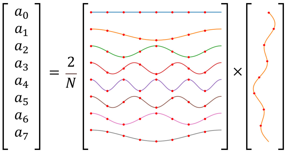
\[ \begin{bmatrix} a_0 \\ a_1 \\ a_2 \\ a_3 \\ a_4 \\ a_5 \\ a_6 \\ a_7 \end{bmatrix} = \frac{2}{8} \begin{bmatrix} 1 & 1 & 1 & 1 & 1 & 1 & 1 & 1 \\ 1 & \frac{1}{\sqrt{2}} & 0 & -\frac{1}{\sqrt{2}} & -1 & -\frac{1}{\sqrt{2}} & 0 & \frac{1}{\sqrt{2}} \\ 1 & 0 & -1 & 0 & 1 & 0 & -1 & 0 \\ 1 & -\frac{1}{\sqrt{2}} & 0 & \frac{1}{\sqrt{2}} & -1 & \frac{1}{\sqrt{2}} & 0 & -\frac{1}{\sqrt{2}} \\ 1 & -1 & 1 & -1 & 1 & -1 & 1 & -1 \\ 1 & -\frac{1}{\sqrt{2}} & 0 & \frac{1}{\sqrt{2}} & -1 & \frac{1}{\sqrt{2}} & 0 & -\frac{1}{\sqrt{2}} \\ 1 & 0 & -1 & 0 & 1 & 0 & -1 & 0 \\ 1 & \frac{1}{\sqrt{2}} & 0 & -\frac{1}{\sqrt{2}} & -1 & -\frac{1}{\sqrt{2}} & 0 & \frac{1}{\sqrt{2}} \end{bmatrix} \times \begin{bmatrix} \frac{3-\sqrt{2}}{\sqrt{2}} \\ \frac{2+2\sqrt{2}}{\sqrt{2}} \\ \frac{3-3\sqrt{2}}{\sqrt{2}} \\ \frac{2-\sqrt{2}}{\sqrt{2}} \\ \frac{-3-\sqrt{2}}{\sqrt{2}} \\ \frac{-2-4\sqrt{2}}{\sqrt{2}} \\ \frac{-3+\sqrt{2}}{\sqrt{2}} \\ \frac{-2-\sqrt{2}}{\sqrt{2}} \end{bmatrix} = \begin{bmatrix} -2 \\ \frac{3}{2}\sqrt{2} \\ 0 \\ 0 \\ 0 \\ 0 \\ 0 \\ \frac{3}{2}\sqrt{2} \end{bmatrix} \]
The matrix representation for sine-weighted coefficients is given by:
\[ \begin{bmatrix} b_0 \\ b_1 \\ b_2 \\ b_3 \\ b_4 \\ b_5 \\ b_6 \\ b_7 \end{bmatrix} = \frac{2}{N} \begin{bmatrix} \sin\left(2\pi n \cdot \frac{0}{8}\right) \\ \sin\left(2\pi n \cdot \frac{1}{8}\right) \\ \sin\left(2\pi n \cdot \frac{2}{8}\right) \\ \sin\left(2\pi n \cdot \frac{3}{8}\right) \\ \sin\left(2\pi n \cdot \frac{4}{8}\right) \\ \sin\left(2\pi n \cdot \frac{5}{8}\right) \\ \sin\left(2\pi n \cdot \frac{6}{8}\right) \\ \sin\left(2\pi n \cdot \frac{7}{8}\right) \end{bmatrix} \times \begin{bmatrix} x(0) \\ x(1) \\ x(2) \\ x(3) \\ x(4) \\ x(5) \\ x(6) \\ x(7) \end{bmatrix} \]
The figure below visually represents the computation of sine coefficients using the DFT matrix.
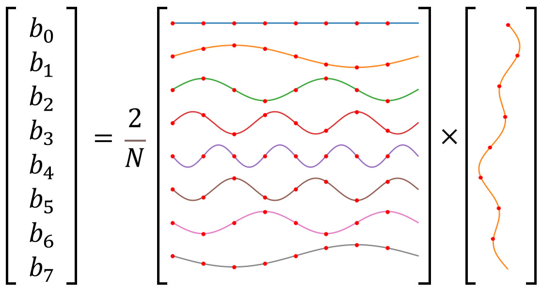
\[ \begin{bmatrix} b_0 \\ b_1 \\ b_2 \\ b_3 \\ b_4 \\ b_5 \\ b_6 \\ b_7 \end{bmatrix} = \frac{2}{8} \begin{bmatrix} 0 & 0 & 0 & 0 & 0 & 0 & 0 & 0 \\ 0 & \frac{1}{\sqrt{2}} & 1 & \frac{1}{\sqrt{2}} & 0 & -\frac{1}{\sqrt{2}} & -1 & -\frac{1}{\sqrt{2}} \\ 0 & 1 & 0 & -1 & 0 & 1 & 0 & -1 \\ 0 & \frac{1}{\sqrt{2}} & -1 & \frac{1}{\sqrt{2}} & 0 & -\frac{1}{\sqrt{2}} & 1 & -\frac{1}{\sqrt{2}} \\ 0 & 0 & 0 & 0 & 0 & 0 & 0 & 0 \\ 0 & -\frac{1}{\sqrt{2}} & 1 & -\frac{1}{\sqrt{2}} & 0 & \frac{1}{\sqrt{2}} & -1 & \frac{1}{\sqrt{2}} \\ 0 & -1 & 0 & 1 & 0 & -1 & 0 & 1 \\ 0 & -\frac{1}{\sqrt{2}} & -1 & -\frac{1}{\sqrt{2}} & 0 & \frac{1}{\sqrt{2}} & 1 & \frac{1}{\sqrt{2}} \end{bmatrix} \times \begin{bmatrix} \frac{3-\sqrt{2}}{\sqrt{2}} \\ \frac{2+2\sqrt{2}}{\sqrt{2}} \\ \frac{3-3\sqrt{2}}{\sqrt{2}} \\ \frac{2-\sqrt{2}}{\sqrt{2}} \\ \frac{-3-\sqrt{2}}{\sqrt{2}} \\ \frac{-2-4\sqrt{2}}{\sqrt{2}} \\ \frac{-3+\sqrt{2}}{\sqrt{2}} \\ \frac{-2-\sqrt{2}}{\sqrt{2}} \end{bmatrix} = \begin{bmatrix} 0 \\ \frac{3}{2}\sqrt{2} \\ 0 \\ 2 \\ 0 \\ -2 \\ 0 \\ -\frac{3}{2}\sqrt{2} \end{bmatrix} \]
Input signal restoration#
The original discrete signal can be reconstructed as:
\[ x(n) = \frac{a_0}{2} + \sum_{k=1}^{N-1} \left( b_k \sin\left(\frac{2\pi k}{N} n\right) + a_k \cos\left(\frac{2\pi k}{N} n\right) \right) \]
The DC component, represented by the coefficient \( a_0 \), is:
\[ \text{DC} = \frac{a_0}{2} = \frac{-2}{2} = -1 \]
For each frequency component \( f_k \):
-
The amplitude is given by:
\[ A_k = \sqrt{a_k^2 + b_k^2} \]
-
The phase is given by:
\[ \varphi_k = \tan^{-1}\left(\frac{a_k}{b_k}\right) \]
The following table summarizes the reconstructed parameters of the input signal:
| \(k\) | \(f_k\) | \(a_k\) | \(b_k\) | \(A_k\) | \(\varphi_k\) |
|---|---|---|---|---|---|
| 0 | 0Hz | -2 | 0 | -1 | - |
| 1 | 1Hz | \(\dfrac{3}{2}\sqrt{2}\) | \(\dfrac{3}{2}\sqrt{2}\) | 3 | \(\dfrac{\pi}{4}\) |
| 2 | 2Hz | 0 | 0 | 0 | - |
| 3 | 3Hz | 0 | 2 | 2 | 0 |
| 4 | -4Hz | 0 | 0 | 0 | - |
| 5 | -3Hz | 0 | -2 | 2 | 0 |
| 6 | -2Hz | 0 | 0 | 0 | - |
| 7 | -1Hz | \(\dfrac{3}{2}\sqrt{2}\) | \(-\dfrac{3}{2}\sqrt{2}\) | 3 | \(-\dfrac{\pi}{4}\) |
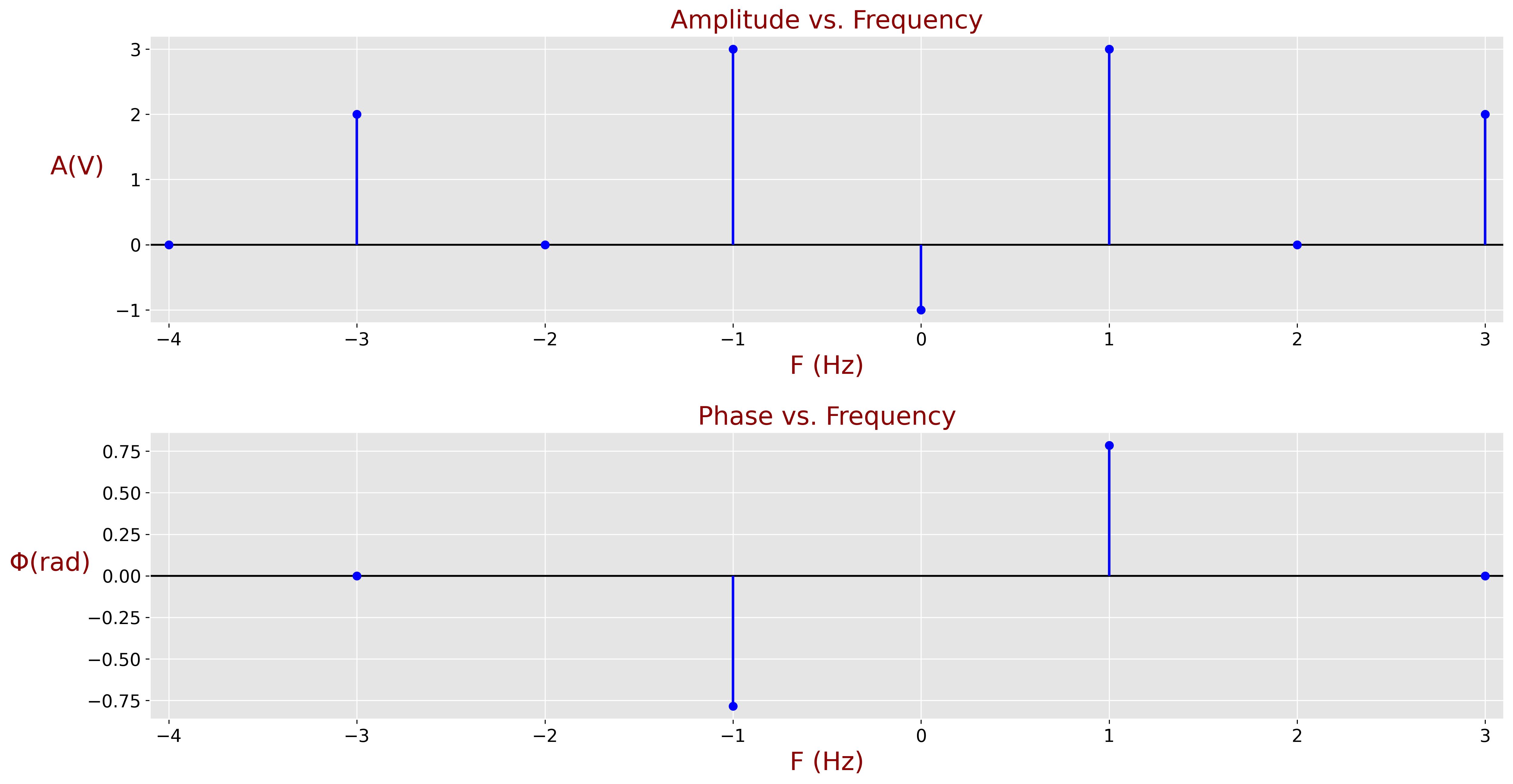
We have successfully reconstructed the DC component, the 1Hz component, and the 3Hz component of the input signal.
However, the results also include negative frequencies that were not explicitly present in the input signal. This occurs because when a signal is correlated with its opposite, it results in a negative correlation. Consequently, the phase of the negative frequency components is opposite to that of the corresponding positive frequency components.
The plot below describes the amplitudes and the phases of reconstructed frequency components.
You can find MATLAB, Python, and C implementation of this example in the DFT Example Software Implementation section.